Maximum Flow Linear Program¶

Definition¶

For the course network with only outgoing source edges and only incoming sink edges, the maximum flow LP (linear program) uses continuous variables $x_{ij}$ and solves

\begin{aligned} \max\quad &\sum_jx_{sj}\\ \text{subject to}\quad &\sum_jx_{ji}=\sum_jx_{ij}\quad(i\ne s,t),\\ &0\le x_{ij}\le c_{ij}\quad\text{for every directed edge }(i,j). \end{aligned}

Here $c_{ij}$ is the edge capacity and sums run over existing edges.

Interpretation¶

The maximum flow LP writes the maximum flow problem as an ordinary linear program: one continuous decision variable per edge, the capacities and the flow balances as linear constraints, and the flow leaving the source as the objective.

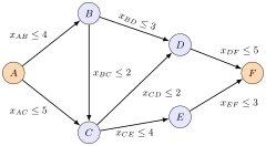
A network from A to F with an upper bound on the flow variable of each edge, x ij at most its capacity.

Each edge label in the figure is one capacity constraint, such as $x_{AB}\le4$ $4$ . Together with $x_{ij}\ge0$ and one balance equation for each of $B$ , $C$ , $D$ and $E$ , these constraints form the whole model. The two edges into $F$ have capacities $5$ and $3$ , so no feasible flow can deliver more than $8$ ; the Examples report that $8$ is attained.

Each part has its own role. The balance equations say that intermediate vertices pass flow on without creating or losing any. They are not imposed at the source and the sink: the source has only outgoing edges, so balance there would force all its edges to carry zero flow. The objective counts only the flow leaving the source, which equals the flow arriving at the sink once all balances hold.

Because the model is an LP, the simplex method or Excel Solver can solve it, as an alternative to the augmenting path algorithm. The same pattern of conservation equations returns in the shortest path formulation, where one unit of flow is sent from origin to destination.

Key Results¶

Source outflow equals sink inflow by summing conservation equations.
No binary selection variable is needed: an edge may carry any feasible flow amount.
The formulation combines the capacity and flow-conservation conditions of the maximum flow problem.

Examples¶

In the figure, maximize $x_{AB}+x_{AC}$ with the displayed edge capacities. The intermediate balances are

\begin{aligned}x_{AB}&=x_{BC}+x_{BD},\\x_{AC}+x_{BC}&=x_{CD}+x_{CE},\\x_{BD}+x_{CD}&=x_{DF},\\x_{CE}&=x_{EF}.\end{aligned}

The optimum is 8. For a maximum-flow formulation with integer capacities, an integral optimal flow exists; this is a property of this network formulation, not of arbitrary LPs with integer data.

In the course example network with source $S$ , the objective is $x_{SA}+x_{SB}$ $x_{S B}$ .
At vertex $A$ of that network, conservation is $x_{SA}=x_{AB}+x_{AC}+x_{AD}$ $x_{A D}$ .

Prerequisites¶

Sources¶

OR Modelling · Week 5

Aliases: maximum flow LP, max-flow LP Symbols: sum

Last updated: 22 October 2026 19:04