Sensitivity Analysis¶

Definition¶

Sensitivity analysis examines how changes in model parameters affect an LP's optimal solution and optimal value. The course studies changes to objective coefficients and resource right-hand sides using final simplex tableaux and Excel sensitivity reports.

Interpretation¶

Sensitivity analysis asks how strongly the answer of an LP depends on its input numbers. Inputs may be estimates, and additional resources may be purchasable, so it matters whether the current decision remains suitable after an input changes and how the optimal value responds, without solving the problem again from scratch.

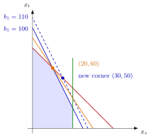
The feasible pentagon with the optimal corner (20, 60), and the finishing constraint shifted outwards so that the optimum moves to the new corner (30, 50).

The figure shows a right-hand-side change in the Giapetto model. Raising the finishing hours from $100$ to $110$ shifts the finishing line outwards, and the optimum moves from $(20,60)$ to $(30,50)$ , where the same two constraints, finishing and carpentry, still cross. The optimal value rises from $180$ to $190$ : $1$ per added hour, the shadow price.

The two kinds of change act differently on the picture. An objective coefficient changes only the slope of the objective line; the feasible region stays the same, so the optimal corner stays put until the slope passes that of an edge, as the objective coefficient range describes. A right-hand side moves a constraint line parallel to itself, so the region changes and the optimal point moves, while the same constraints stay binding over the RHS sensitivity range. For variables that are $0$ at the optimum, the reduced cost gives the cost of forcing them into the plan.

A common slip is to combine several ranges from an Excel sensitivity report as if they still held together: each range assumes that all other data stay fixed.

Key Results¶

The reported allowable ranges apply to one parameter change at a time.
Changing an objective coefficient can preserve the solution vector while changing profit.
Changing a right-hand side can change the solution vector even while the same basis and shadow prices remain valid.
Outside a valid range, reoptimization may be needed.

Examples¶

For the illustrated objective with $c_2>0$ $0$ , $(20,60)$ remains optimal when $1\le c_1/c_2\le2$ $2$ . Changing the finishing right-hand side (RHS) from 100 to 110 instead moves the optimum to $(30,50)$ while preserving the basis. Within the applicable one-parameter range, $\Delta z=y_i^*\Delta b_i$ $y_{i}^{*} Δ b_{i}$ .

A change in banana ice-cream profit from 0.95 to 0.92 leaves the given production plan optimal.
Losing three gallons of cream changes the ice-cream quantities and reduces optimal profit by 3.

Prerequisites¶

Sources¶

OR Modelling · Week 3

Aliases: post-optimality analysis, postoptimal analysis Symbols: delta

Last updated: 20 October 2026 03:02