Job Sequencing Model¶

Definition¶

The job sequencing model orders jobs on one machine, each processed without interruption once started (nonpreemptive), to minimize total weighted tardiness penalties. Let $s_i\ge0$ be job $i$ 's start, $p_i$ its duration, $d_i$ its due date, $T_i\ge0$ its tardiness, and $w_i$ its penalty rate. Minimize $\displaystyle \sum_iw_iT_i$ subject to $T_i\ge s_i+p_i-d_i$ $d_{i}$ . For each pair $i<j$ $j$ , impose

s_i+p_i\le s_j+M(1-y_{ij}),\qquad s_j+p_j\le s_i+My_{ij},\qquad y_{ij}\in\{0,1\}.

Here $y_{ij}=1$ means $i$ precedes $j$ , and $M$ must be valid for the scheduling horizon.

Interpretation¶

The job sequencing model decides in which order jobs run on a single machine so that lateness costs as little as possible. Pairwise order choices keep two jobs from occupying the machine at the same time, and tardiness variables charge for finishing after the due date but not for finishing early.

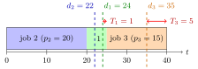
A timeline with three jobs processed one after another, job 2, job 1 and job 3, with vertical lines at their due dates and the tardiness of jobs 1 and 3 marked.

The timeline shows the sequence $2,1,3$ from the Examples: job 2 runs from $0$ to $20$ , job 1 from $20$ to $25$ and job 3 from $25$ to $40$ . Job 2 finishes before $d_2=22$ $22$ , so $T_2=0$ $0$ ; job 1 finishes one unit after $d_1=24$ and job 3 five units after $d_3=35$ $35$ , which gives the marked $T_1=1$ and $T_3=5$ and the cost $189$ .

For each pair the two order constraints are an either-or pair. If $y_{ij}=1$ $1$ , the first says that job $i$ finishes before job $j$ starts, and the second is switched off by $M$ ; if $y_{ij}=0$ $0$ , the roles are swapped. One binary variable per pair suffices because two non-overlapping jobs run in one of only two orders. With continuous start times, the model is a mixed integer program.

The tardiness constraint $T_i\ge s_i+p_i-d_i$ with $T_i\ge0$ only bounds $T_i$ from below. Because the objective minimizes $\displaystyle \sum_iw_iT_i$ with positive rates $w_i$ , an optimal solution pushes each $T_i$ down to the larger of $0$ and $s_i+p_i-d_i$ $d_{i}$ . Writing $T_i=s_i+p_i-d_i$ instead is a common slip: an early job would then get negative tardiness, rewarding earliness, or, with $T_i\ge0$ kept, be ruled out altogether.

Key Results¶

For the supplied three jobs, total processing time is 40; a no-idle schedule starts at zero and lies within that horizon.
Nonnegative penalty rates make unnecessary idle time avoidable.
The formulation applies the either-or technique to the exercise's three jobs.

Examples¶

The course has processing times $(5,20,15)$ , due dates $(24,22,35)$ and penalty rates $(19,12,34)$ for jobs 1, 2, 3.
Sequence $2,1,3$ completes at 20, 25, 40 and incurs $12(0)+19(1)+34(5)=189$ $189$ .

Prerequisites¶

Task Quota Assignment

Sources¶

OR Modelling · Week 3

Aliases: single-machine weighted tardiness problem Symbols: element of, sum

Last updated: 27 October 2026 11:52