Silver-Meal Heuristic¶

Definition¶

The Silver-Meal heuristic chooses consecutive periods to cover with each order when the variable unit ordering cost is constant and identical across periods. For an order in period $i$ covering through $t$ , define

\begin{gathered} TC(i,t)=K_i+\sum_{j=i+1}^tD_j\sum_{k=i}^{j-1}h_k,\\ TCU(i,t)=\frac{TC(i,t)}{t-i+1}. \end{gathered}

Starting at the first uncovered period, extend coverage while average cost decreases, select the first local minimum, order $\displaystyle \sum_{j=i}^{t^*}D_j$ , and restart at $i=t^*+1$ $1$ . Stop at the horizon; on a flat tie, selecting the first local minimum is the convention used here.

Interpretation¶

The heuristic decides how many periods one order should cover by looking at the average cost per covered period. Covering more periods spreads the setup cost $K_i$ over more periods but adds holding cost for the units carried forward; the rule stops extending the order when this average starts to rise.

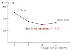
The cost per covered period for orders covering one to four periods: it falls to a first minimum at three periods and then rises, so the order covers three periods.

For an order placed in period 1, covering only period 1 costs $K$ alone, $50$ per period. Covering periods 1 and 2 lowers the average to $35$ and covering periods 1 to 3 lowers it to $30$ , but adding period 4 raises it to $33$ . The first local minimum is $t^*=3$ $3$ , so the first order covers $D_1+D_2+D_3$ and the method restarts at period 4.

In $TC(i,t)$ , the demand $D_j$ of a later period $j$ is held from period $i$ until period $j$ , which is why it is multiplied by $h_i+\dots+h_{j-1}$ $h_{j - 1}$ . Dividing by $t-i+1$ makes covers of different lengths comparable. Purchasing cost is left out because, with a common unit price, it is the same for every policy that meets all demand.

The rule is greedy: it fixes each order before looking at later periods and stops at the first rise, so this heuristic can miss a cheaper pattern. In the second listed Example it costs $169$ , against $152$ for the optimum found by dynamic programming. Its orders always arrive at zero stock and cover whole periods, the form described by the zero-inventory ordering property.

Key Results¶

Purchasing cost is omitted from the comparisons because the common unit price gives the same total for every complete demand-covering policy.
Add that constant purchasing cost when reporting a total that includes it.
At the start or end of the horizon, use only available neighbouring average-cost comparisons.

Examples¶

The figure’s first order covers $D_1+D_2+D_3$ $D_{3}$ ; the rule then restarts at period 4. The displayed values are illustrative rather than the complete course exercise data.

The six-period video orders $(32,0,0,20,13,25)$ , with setup and holding cost 122.
Week 6 practice 4 orders $(9,22,0,0)$ and costs 169 including purchases; the exact DP cost is 152.

Prerequisites¶

Sources¶

OR Modelling · Week 6

Aliases: least period cost heuristic, Silver-Meal method Symbols: sum

Last updated: 20 October 2026 03:02