Dynamic Programming¶

Definition¶

Dynamic programming (DP) decomposes an optimization problem into related subproblems and computes their optimal values recursively. A state records the information needed to connect stages, and the optimum for a smaller subproblem becomes an input to the next calculation.

Interpretation¶

Dynamic programming solves a problem made of a sequence of decisions stage by stage. The cost of the remaining decisions depends only on the current state, not on how that state was reached, so the best value of each state is computed once and reused, instead of once for every complete policy that passes through it.

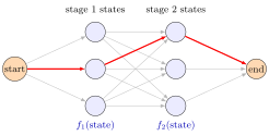
A staged network from start through two stages of three states each to end, with all arrows between stages and the optimal route highlighted.

Each column is a stage, each circle a state, and every route from start to end is one complete policy. Listing routes repeats the same arrow costs many times: with $m$ stages of three states there are $3^m$ routes but fewer than $9m$ arrows. The forward calculation stores one value $f_1$ per stage-1 state, computes each $f_2$ from the three arrows entering it, and reaches the end after looking at every arrow once.

A DP model needs a state that contains everything the later stages depend on. In the dynamic lot-size model the stage is the period and the state is the stock carried into the next period, as in the lot-size recursion. If the state leaves out relevant information, histories that should be treated differently are merged and the recursion can give a wrong answer.

The cheapest policy is a cheapest route from start to end through the staged network, which links DP to the shortest path problem. Unlike a heuristic such as the Silver-Meal heuristic, DP guarantees an optimal solution.

Key Results¶

Specify the state, decision, transition, cost, boundary conditions, and recursion.
Store minimizing decisions as well as costs to reconstruct an optimal policy.
Keep every minimizing decision if all optimal policies are required.

Examples¶

For the figure’s forward calculation, each incoming arrow contributes its transition cost plus the preceding state value: $f_2(\text{state})=\min_{\text{incoming arrows}}\{\text{arrow cost}+f_1(\text{previous state})\}$ $f_{1} (previous state)}$ . The red arrows record the minimizing decisions used to reconstruct the policy.

$f_i(x_{i+1})$ records the least cost through period $i$ for a specified ending inventory.
The three-period calculation finds $f_3(0)=79$ and then traces decisions backward.

Prerequisites¶

Sources¶

OR Modelling · Week 6

Aliases: DP

Last updated: 20 October 2026 03:02