EOQ with Planned Shortages¶

Definition¶

The EOQ model with planned shortages allows all unmet demand to be backordered until instantaneous replenishment. With constant $D>0$ $0$ , setup $K>0$ $0$ , holding rate $h>0$ $0$ , and shortage cost (backlog penalty) $p>0$ $0$ , choose batch size $y>0$ and stock just after replenishment $0\le s\le y$ $y$ . Maximum backlog is $y-s$ $s$ , and

TCU(y,s)=\frac{KD}{y}+\frac{hs^2}{2y}+\frac{p(y-s)^2}{2y}.

The optimum is

\begin{aligned} y^*&=\sqrt{\frac{2KD}{h}}\sqrt{\frac{p+h}{p}},\\ s^*&=\sqrt{\frac{2KD}{h}}\sqrt{\frac{p}{p+h}}. \end{aligned}

Interpretation¶

This model lets stock run below zero on purpose: customers who arrive when the shelf is empty wait, and are served as soon as the next batch arrives. Waiting is charged at rate $p$ per unit per unit time, so the model trades waiting customers against the cost of holding stock.

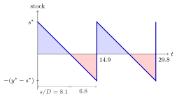
A sawtooth stock level that falls below zero in each cycle, with the positive parts and the backlogged parts shaded differently, before each new order arrives.

In the phone example, each batch of $y^*\approx29.79$ first clears the backlog of about $13.54$ and leaves $s^*\approx16.25$ phones on hand. Stock is positive for about $8.1$ days (blue) and backlogged for about $6.8$ days (red) of each $14.9$ -day cycle. The fraction of time with stock is $s^*/y^*=6/11=p/(p+h)$ $h)$ .

Two decisions are made now: the batch size $y$ and the stock $s$ left after the backlog is cleared. Holding cost is charged only on the blue triangles, so the average stock over a whole cycle is $s^2/(2y)$ , and shortage cost is charged on the red triangles. Short periods of shortage save holding cost, which is why some backlog pays off whenever $p$ is finite.

The factor $\sqrt{(p+h)/p}$ links the model to the classical EOQ: the larger $p$ , the closer the factor is to $1$ . With $p=600$ instead of $6$ , $y^*\approx22.09$ $22.09$ , almost the classical $22$ , with a tiny backlog. A common slip is to treat backlog as lost sales: here every waiting customer is served, so the ordering cycle is still $y/D$ .

Key Results¶

Order $y^*$ when backlog reaches $y^*-s^*$ $s^{*}$ .
Ordering cycle length is $y^*/D$ ; the fraction of time without shortage is $p/(p+h)$ $h)$ .
The stock-phase mean $s/2$ is not the whole-cycle average; the latter is $s^2/(2y)$ .
For finite positive $p$ , the optimal batch is larger than the classical EOQ.

Examples¶

In the illustrated phone example, $D=2$ per day, $K=605$ $605$ , $h=5$ per phone per day and $p=6$ per backlogged phone per day give $y^*=22\sqrt{11/6}\approx29.79$ and $s^*=22\sqrt{6/11}\approx16.25$ $16.25$ . Order when the backlog reaches $y^*-s^*\approx13.54$ $13.54$ . The cycle lasts about $14.9$ days: stock is positive for about $8.1$ days and backlogged for about $6.8$ days, with stock-positive fraction $6/11$ .
With $p=h$ $h$ , the model is out of stock for half the cycle.

Prerequisites¶

Sources¶

OR Modelling · Week 5

Aliases: EOQ with backorders, EOQ with backlogging, planned backorder model Symbols: square root

Last updated: 20 October 2026 03:02