Classical EOQ Model¶

Definition¶

The classical EOQ model, based on the economic order quantity (EOQ), assumes deterministic constant demand rate $D>0$ $0$ , instantaneous batch replenishment, no shortages, fixed setup cost $K>0$ per order, and holding cost $h>0$ per unit per unit time. A constant unit purchasing price can be excluded when optimizing. For batch size $y>0$ $0$ , relevant total cost per unit time (TCU) is

TCU(y)=\frac{KD}{y}+\frac{hy}{2}.

Interpretation¶

The classical EOQ model is the simplest inventory policy model: demand is steady and known, so stock follows a fixed repeating pattern, and only the batch size $y$ remains to be chosen. Large batches mean few setups but much stock; small batches mean the reverse.

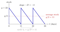
A sawtooth stock level that drops from 22 to 0 at a constant rate and is refilled every 11 days, with a horizontal line at the average stock 11.

Stock starts at $y=22$ and falls with slope $-D=-2$ $- 2$ , reaching zero after $t_0=y/D=11$ days, when the next batch arrives at once. The dashed line at $y/2=11$ is the average stock, which fixes the holding cost rate $hy/2$ .

Each assumption shapes the picture. Constant demand makes the falling parts straight lines. Instantaneous replenishment makes the jumps vertical. Because shortages are not allowed and ordering earlier would only add holding cost, the next batch arrives exactly when stock reaches zero. A constant unit price adds the same purchasing cost per unit time for every $y$ , so it can be left out of $TCU(y)$ when choosing $y$ .

Minimizing $TCU(y)$ gives the economic order quantity. Relaxing one assumption at a time gives the other models of this week: a delay between ordering and delivery in EOQ with lead times, backlogged demand in EOQ with planned shortages, and order-size discounts in EOQ with price breaks. In the last model, $TCU(y)$ without purchasing cost is no longer enough, since the unit price then depends on $y$ .

Key Results¶

Average stock is $y/2$ and ordering cycle length is $y/D$ .
The cost is strictly convex for positive $y$ .
The model optimizes a continuous order quantity; discrete purchasing units require checking feasible nearby quantities.
Using a mean demand to approximate stochastic demand does not incorporate its variability.

Examples¶

The phone data $D=2$ $2$ , $K=605$ $605$ , $h=5$ give an optimal batch of 22.
The exercise uses average weekly demand 100 while explicitly omitting its standard deviation 10 from the EOQ calculation.

Prerequisites¶

Sources¶

OR Modelling · Week 5

Aliases: Harris-Wilson model, Economic order quantity model, basic EOQ model, Wilson EOQ model Keywords: EOQ model

Last updated: 20 October 2026 03:02