Variance and Standard Deviation¶

Definition¶

Let $X$ be a random variable with $\mathbb{E}[X^2]<\infty$ $\infty$ , and let $\mu=\mathbb{E}X$ $E X$ . The variance of $X$ is

\operatorname{Var}(X)=\mathbb{E}[(X-\mu)^2]=\mathbb{E}[X^2]-\mu^2,

and the standard deviation is $\sigma_X=\sqrt{\operatorname{Var}(X)}$ $Var (X)$ .

Interpretation¶

Variance measures how far the values of $X$ typically lie from the mean $\mu=\mathbb{E}X$ $E X$ : it is the probability-weighted average of the squared distance $(X-\mu)^2$ $μ)^{2}$ . The standard deviation, its square root, measures the same spread in the original units of $X$ .

Two normal densities with the same mean, a narrow one with standard deviation 1 and a wide one with standard deviation 2, with arrows showing one standard deviation for each.

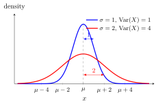
The figure shows two bell-shaped distributions with the same mean $\mu$ . The narrow curve has standard deviation $1$ and the wide one standard deviation $2$ ; the arrows run from $\mu$ to $\mu+\sigma$ for each curve. Doubling the standard deviation multiplies the variance by four, from $1$ to $4$ , because variance is measured in squared units.

Each part of $\mathbb{E}[(X-\mu)^2]$ has a role. Centring at $\mu$ makes the measure ignore location: adding a constant to $X$ moves $\mu$ by the same amount, so $\operatorname{Var}(a+X)=\operatorname{Var}(X)$ $Var (X)$ . Squaring makes deviations on both sides count as positive and weights large deviations heavily. The second formula in the definition, $\mathbb{E}[X^2]-\mu^2$ $μ^{2}$ , is usually quicker: for a Bernoulli variable $X^2=X$ $X$ , so $\mathbb{E}[X^2]=p$ and $\operatorname{Var}(X)=p-p^2=p(1-p)$ $p)$ .

Scaling does not act linearly on variance: $\operatorname{Var}(bX)=b^2\operatorname{Var}(X)$ $b^{2} Var (X)$ , while the standard deviation is multiplied by $|b|$ , so $-X$ has the same variance as $X$ . For independent variables the variances add, as on the page on sums of independent random variables, but the standard deviations do not. When $\sigma_X>0$ $0$ , dividing $X-\mu$ by $\sigma_X$ gives a variable with mean $0$ and variance $1$ , which returns later as standardization. A constant variable has $\sigma_X=0$ and cannot be standardized by this division.

Key Results¶

$\operatorname{Var}(a+bX)=b^2\operatorname{Var}(X)$ $b^{2} Var (X)$ .
$\operatorname{Var}(X)=0$ if and only if $X=\mathbb{E}X$ almost surely, that is, $\mathbb{P}(X=\mathbb{E}X)=1$ $1$ .

Examples¶

For $\operatorname{Bern}(0.3)$ , the variance is $0.3(0.7)=0.21$ $0.21$ .
If $\operatorname{Var}(X)=4$ $4$ , then $\operatorname{Var}(5-3X)=36$ and its standard deviation is $6$ .

Prerequisites¶

Sources¶

Probability Theory for EOR · Week 4
Nicky van Foreest · Probability Distributions · Refresher

Aliases: Var, SD, second central moment Keywords: variance, standard deviation Symbols: infinity, mu, sigma, square root

Last updated: 27 October 2026 11:52