Universality of the Uniform and CDF Realizability¶

Theorem¶

Let $F\colon\mathbb{R}\to[0,1]$ be nondecreasing and right-continuous, with $\displaystyle\lim_{x\to-\infty}F(x)=0$ and $\displaystyle\lim_{x\to\infty}F(x)=1$ $1$ . Let $U\sim\operatorname{Unif}(0,1)$ and define $Q(u)=\inf\{x\colon F(x)\ge u\}$ for $0<u<1$ $1$ . Then $X=Q(U)$ satisfies

\mathbb{P}(X\le x)=F(x)\quad\text{for every }x.

Thus every function satisfying the CDF conditions is realizable as a distribution, and a uniform input can generate that distribution. The construction allows jumps and flat portions of $F$ .

Interpretation¶

A uniform draw selects a probability level; the quantile function converts it into an outcome. This both proves that valid CDFs describe genuine random variables and provides inverse transform simulation.

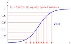
An S-shaped CDF with equally spaced probabilities on the vertical axis mapped across and down to quantiles on the horizontal axis, which bunch together where the curve is steep.

The equally spaced probability levels map to quantiles $x=Q(u)$ $Q (u)$ . These quantiles are closer together where $F$ is steep, illustrating how a uniform input produces the target distribution.

The uniform distribution on $(0,1)$ assigns probability $v$ to the interval $(0,v]$ . The quantile construction turns $\{Q(U)\le x\}$ into $\{U\le F(x)\}$ $F (x)}$ , so that probability becomes $F(x)$ .

Key Results¶

The monotonicity, right-continuity, and endpoint-limit conditions are necessary and sufficient for a function to be a CDF.
For $0<u<1$ $1$ , $Q(u)\le x$ exactly when $u\le F(x)$ $F (x)$ , so $\mathbb{P}(Q(U)\le x)=\mathbb{P}(U\le F(x))=F(x)$ $F (x)$ .
Conversely, if $X$ has a continuous CDF $F$ , then $F(X)\sim\operatorname{Unif}(0,1)$ $Unif (0, 1)$ ; this direction is the probability integral transform. It fails when $F$ has jumps, because $F(X)$ then takes some values with positive probability.

Examples¶

For the step CDF $F(x)=0$ when $x<c$ and $F(x)=1$ when $x\ge c$ $c$ , $Q(u)=c$ and the construction gives $X=c$ almost surely, that is, with probability $1$ .
For $F(x)=0$ when $x<0$ and $F(x)=1-\mathrm{e}^{-2x}$ when $x\ge0$ $0$ , the construction gives $X=-\log(1-U)/2\sim\operatorname{Exp}(2)$ $Exp (2)$ .

Prerequisites¶

Sources¶

Probability Theory for EOR · Week 5
Nicky van Foreest · Probability Distributions · Week 2

Aliases: CDF realizability Keywords: probability integral transform, inverse transform sampling, inverse transformation method, Smirnov transform, inverse transform method, Universality of the Uniform, Realizability of a CDF Symbols: infinity, real numbers

Last updated: 17 October 2026 21:53