Mixture Distribution¶

Definition¶

Let $Z$ be a random index taking finitely or countably many values, and let the conditional distribution of $X$ given $Z=i$ be specified for each $i$ with $\mathbb{P}(Z=i)>0$ $0$ . The distribution of $X$ is a mixture distribution if it is obtained by averaging these conditional distributions using the probabilities of the values of $Z$ . A continuous mixing index instead requires integration against its mixing distribution.

Interpretation¶

A mixture describes a population made of hidden groups. To draw $X$ , first pick a group $Z$ at random, then draw $X$ from that group's distribution; the distribution of $X$ is the weighted average of the group distributions, with the group probabilities as weights.

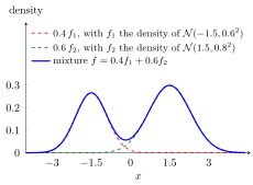
Two weighted normal densities, centred at minus 1.5 and 1.5, and their sum, a mixture density with two peaks.

The figure has two groups with weights $\mathbb{P}(Z=1)=0.4$ and $\mathbb{P}(Z=2)=0.6$ $0.6$ . The dashed curves are the group curves $f_1$ and $f_2$ , centred at $-1.5$ and $1.5$ and already multiplied by their weights; the solid curve is their sum $0.4f_1+0.6f_2$ $0.6 f_{2}$ . These curves are densities: areas under them are probabilities. Each group curve has one peak, but the mixture has two, because the groups lie far apart compared with their spread.

The averaging is the law of total probability for the partition of the sample space by the value of $Z$ : for every set $B$ of values,

\mathbb{P}(X\in B)=\sum_i\mathbb{P}(Z=i)\,\mathbb{P}(X\in B\mid Z=i).

Each conditional probability $\mathbb{P}(X\in B\mid Z=i)$ describes one group. A discrete example: a coin is fair with probability $\tfrac{1}{2}$ and two-headed with probability $\tfrac{1}{2}$ ; for one toss of this coin, with $X=1$ for heads, $\mathbb{P}(X=1)=\tfrac{1}{2}\cdot\tfrac{1}{2}+\tfrac{1}{2}\cdot1=\tfrac{3}{4}$ $\frac{3}{4}$ .

A mixture is not a sum of random variables. $X$ comes from one group, chosen at random, whereas a sum adds a value from each group. In the figure the mixture puts its probability near $-1.5$ and near $1.5$ ; adding one value from each group would instead give values near $0$ .

Key Results¶

A mixture distribution is a weighted average of component distributions.
The weights are nonnegative and sum to one.
Mixtures can produce multimodal shapes even when each component is unimodal.

Examples¶

Customer spending can be modelled as a mixture of business and leisure customer distributions.
Machine lifetime may be a mixture of lifetimes from old and new machines.
Exam scores can form a mixture if two preparation groups are present.

Prerequisites¶

Sources¶

Probability Theory for EOR · Week 3

Aliases: mixture of distributions, distribution mixture Symbols: element of, sum

Last updated: 20 October 2026 03:02