Uniform Distribution¶

Definition¶

For real numbers $a<b$ $b$ , a random variable $X$ has the uniform distribution on $(a,b)$ , written $X\sim\operatorname{Unif}(a,b)$ $Unif (a, b)$ , if its density is

f_X(x)=\begin{cases}1/(b-a),&a<x<b,\\0,&\text{otherwise}.\end{cases}

Including the endpoints in the density interval does not change the distribution.

Interpretation¶

The uniform distribution on $(a,b)$ models a value that lies between $a$ and $b$ with no part of that interval favoured: the probability of a subinterval is proportional to its length.

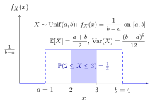
A flat density of height 1/3 on the interval from 1 to 4, with the area between 2 and 3 shaded, equal to 1/3.

With $a=1$ and $b=4$ the density is flat at height $1/(b-a)=1/3$ and zero outside the interval, so the rectangle under it has area $3\cdot\tfrac{1}{3}=1$ $1$ . The shaded strip from $2$ to $3$ has length $1$ and hence probability $\tfrac{1}{3}$ ; every other strip of length $1$ inside $(1,4)$ has the same probability, wherever it is placed.

The mean $(a+b)/2$ is the midpoint of the interval, and the variance $(b-a)^2/12$ depends only on the length, so shifting the interval moves the mean and leaves the variance unchanged. Height and width trade off: a short interval forces a tall density, and for $b-a<1$ the height exceeds $1$ , which is allowed because heights of a continuous random variable are not probabilities. For the same reason each single value has probability $0$ ; "uniform" means equal probability for equal lengths.

$\operatorname{Unif}(0,1)$ is the basic building block. If $U\sim\operatorname{Unif}(0,1)$ $Unif (0, 1)$ , then $a+(b-a)U\sim\operatorname{Unif}(a,b)$ $Unif (a, b)$ , and by the universality of the uniform a suitable function of $U$ , its quantile function, has any prescribed distribution; this is how random numbers with other distributions are simulated. The discrete uniform distribution is the counterpart for finitely many equally likely values.

Key Results¶

$\mathbb{E}X=(a+b)/2$ and $\operatorname{Var}(X)=(b-a)^2/12$ $a)^{2} /12$ .
For $a\le c\le d\le b$ $b$ , $\mathbb{P}(c<X<d)=(d-c)/(b-a)$ $a)$ .

Examples¶

For $X\sim\operatorname{Unif}(2,6)$ $Unif (2, 6)$ , $\mathbb{P}(3<X<5)=2/4=1/2$ $1/2$ .
For $X\sim\operatorname{Unif}(0,1)$ $Unif (0, 1)$ , $\mathbb{E}X=1/2$ and $\operatorname{Var}(X)=1/12$ $1/12$ .

Prerequisites¶

Sources¶

Probability Theory for EOR · Week 5
Nicky van Foreest · Probability Distributions · Week 2

Aliases: continuous uniform distribution, Unif(a,b), rectangular distribution, uniform random variable Keywords: Uniform

Last updated: 20 October 2026 03:02