Memoryless Property
Definition
A nonnegative waiting time is memoryless if, once it has lasted a certain time, the time still to wait has the same distribution as the original waiting time. For a nonnegative integer-valued this means that for all nonnegative integers
For an absolutely continuous nonnegative it means that for all
The conditioning events must have positive probability. The property also works in reverse. Suppose the waiting time is finite with probability and all its tail probabilities are positive. Then a memoryless has a distribution for some (counting the failures before the first success), and a memoryless has an distribution for some . For the first-success distribution, which counts trials and takes the values , the same condition is written with strict tails: for all nonnegative integers .
Interpretation
A memoryless waiting time does not age: having waited for a while says nothing about how much longer the wait will be. A working component with a memoryless lifetime is as good as new.
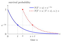
The blue curve is the survival probability of an exponential waiting time. The red dashed curve is the conditional probability of survival given : it starts at at time and is an exact copy of the blue curve shifted to the right by . Its height at equals the height of the blue curve at :
Since is contained in , the condition can be written without conditioning as : the survival probability turns sums of times into products, and that is what forces the exponential form. The discrete version reads the same way: means that the first trials all failed, and given this the number of further failures is again , since the trials are independent.
Most lifetimes with wear do not have it: for , while . The property also does not say that a long wait makes an end "due": after ten failures in independent trials, a success is no more likely than before. It is what makes the Poisson process start afresh at every moment: from any fixed time, the wait for the next arrival is again .
Key Results
- For counting failures, for admissible nonnegative integers .
- For , for .
Examples
- For , .
- For , .
Prerequisites
Related Concepts
- Exponential Distribution
- Geometric Distribution
- First Success Distribution
- Survivor Function
- Poisson Process
Sources
- Probability Theory for EOR · Week 6
- Nicky van Foreest · Probability Distributions · Week 2
Aliases: memorylessness, lack of memory, lack-of-memory property Keywords: Memoryless Symbols: lambda
Last updated: 22 October 2026 19:04
Memoryless PropertyConditional ProbabilityExponential DistributionGeometric DistributionFirst Success DistributionSurvivor FunctionPoisson Process