Gamma Distribution¶

Definition¶

For shape $r>0$ and rate $\lambda>0$ $0$ , $X\sim\operatorname{Gamma}(r,\lambda)$ has density

f_X(x)=\begin{cases}\dfrac{\lambda^r}{\Gamma(r)}x^{r-1}\mathrm{e}^{-\lambda x},&x>0,\\0,&x\le0.\end{cases}

The Gamma Function in the denominator normalizes the density: substituting $z=\lambda x$ makes the unnormalized integral equal to $\Gamma(r)$ , which cancels the denominator.

Interpretation¶

The gamma family extends exponential waiting times. For a positive integer shape $r$ , $\operatorname{Gamma}(r,\lambda)$ is the distribution of a sum of $r$ independent $\operatorname{Exp}(\lambda)$ waits, for example the time until the $r$ -th arrival in a Poisson process with rate $\lambda$ .

Gamma densities with rate 1 and shape r = 1, 2 and 3: the exponential density for r = 1, and humps that move right as r grows, with means 2 and 3.

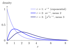
The figure shows three densities with rate $\lambda=1$ $1$ . For $r=1$ the density on $x>0$ is the exponential one, $\mathrm{e}^{-x}$ , with right-hand limit $1$ as $x\downarrow0$ $0$ . The displayed version sets $f_X(0)=0$ $0$ , so its supremum $1$ is approached rather than attained; changing a density at a single point does not change the distribution. For $r=2$ and $r=3$ the factor $x^{r-1}$ pushes the density down to $0$ at the origin, giving a hump with its peak at $x=r-1$ $1$ . The means $r/\lambda=2$ and $3$ move to the right, and the spread grows with the variance $r/\lambda^2$ .

The shape $r$ sets the form of the density through the power $x^{r-1}$ , and the rate $\lambda$ only sets the scale: if $X\sim\operatorname{Gamma}(r,1)$ $Gamma (r, 1)$ , then $X/\lambda\sim\operatorname{Gamma}(r,\lambda)$ $Gamma (r, λ)$ . Non-integer shapes are allowed because the gamma function normalizes the density for every $r>0$ $0$ ; they no longer count exponential waits, but the formulas for mean, variance and MGF stay the same.

The MGF $(\lambda/(\lambda-t))^r$ is the $r$ -th power of the exponential MGF, so the MGF of an independent sum and MGF uniqueness prove the sum property. The same argument shows that independent $\operatorname{Gamma}(r,\lambda)$ and $\operatorname{Gamma}(s,\lambda)$ variables add to $\operatorname{Gamma}(r+s,\lambda)$ $s, λ)$ , provided the rates agree. Some texts use a scale parameter $\theta=1/\lambda$ instead, with mean $r\theta$ ; check the convention before using a formula.

Key Results¶

In shape-rate notation, $\mathbb{E}X=r/\lambda$ and $\operatorname{Var}(X)=r/\lambda^2$ $r / λ^{2}$ .
$M_X(t)=(\lambda/(\lambda-t))^r$ for $t<\lambda$ $λ$ ; shape $r=1$ gives the exponential law.

Examples¶

For shape $r=2$ and rate $\lambda=1$ $1$ , the density is $x\mathrm{e}^{-x}$ on $x>0$ $0$ , the mean is $2$ , and the variance is $2$ .
The sum of three independent $\operatorname{Exp}(2)$ waits has $\operatorname{Gamma}(3,2)$ distribution, with mean $3/2$ and variance $3/4$ .

Prerequisites¶

Sources¶

Probability Distributions · supporting concept

Keywords: Erlang distribution Symbols: gamma, lambda, theta

Last updated: 27 October 2026 11:52