Conditional Expectation Given a Random Variable¶

Definition¶

For integrable $Y$ (that is, $\mathbb{E}|Y|<\infty$ $\infty$ ), the conditional expectation $\mathbb{E}[Y\mid X]$ is a function $g(X)$ of $X$ satisfying the averaging identity $\mathbb{E}[Y\indicator_{\{X\in B\}}]=\mathbb{E}[g(X)\indicator_{\{X\in B\}}]$ for every event $\{X\in B\}$ determined by $X$ . When a conditional PMF or PDF exists,

g(x)=\mathbb{E}[Y\mid X=x]=\begin{cases}\sum_y y\,p_{Y\mid X}(y\mid x), & Y\text{ discrete},\\[4pt] \int_{\mathbb{R}}y\,f_{Y\mid X}(y\mid x)\,\mathrm{d}y, & Y\text{ has a conditional density}.\end{cases}

The sum or integral is selected by the conditional law of $Y$ , not by whether the conditioning variable $X$ is discrete or continuous.

The Expectation calculation averages the possible values of $Y$ under its conditional law. In the continuous case, the weighting function is the Conditional Probability Density Function, not the marginal PDF of $Y$ .

Interpretation¶

Conditioning on a variable produces a new random variable: $\mathbb{E}[Y\mid X]$ is the average of $Y$ predicted from the value of $X$ , and it changes with the value observed. Evaluating it at a fixed value $x$ gives an ordinary number.

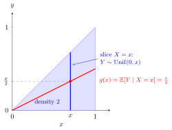
A triangular region with density 2 and a vertical slice at X = x, on which Y is uniform from 0 to x; a line through the slice midpoints shows the conditional mean x/2.

In the illustrated triangular model, with density $2$ on $0<y<x<1$ $1$ , the vertical slice at $X=x$ shows that the conditional distribution of $Y$ given $X=x$ is uniform on $(0,x)$ , with mean $g(x)=x/2$ $x /2$ ; at $x=0.7$ this is the red point at height $0.35$ . Evaluating this function at the random $X$ gives $\mathbb{E}[Y\mid X]=g(X)=X/2$ $X /2$ .

For each fixed $x$ , compute the number $g(x)=\mathbb{E}[Y\mid X=x]$ from the conditional PMF or density, as in the Definition; then substitute the random $X$ . The averaging identity explains what the result is: over every event determined by $X$ , the variable $g(X)$ has the same average as $Y$ . With $B=\mathbb{R}$ it gives $\mathbb{E}[g(X)]=\mathbb{E}Y$ $E Y$ , which is Adam’s law. In the triangle, $\mathbb{E}[X/2]=\tfrac{1}{2}\cdot\tfrac{2}{3}=\tfrac{1}{3}$ $\frac{1}{3}$ , which is indeed $\mathbb{E}Y$ .

For discrete $X$ , the random variable $\mathbb{E}[Y\mid X]$ takes the value $\mathbb{E}[Y\mid X=x]$ on the event $\{X=x\}$ $x}$ , so it collects the numbers $\mathbb{E}[Y\mid A]$ of conditional expectation given an event into one random variable. Its working rules are taking out what is known and the independent case.

Keep three objects apart: $\mathbb{E}Y$ is a number, $\mathbb{E}[Y\mid X=x]$ is a number for each $x$ , and $\mathbb{E}[Y\mid X]$ is a random variable, a function of $X$ .

Key Results¶

$\mathbb{E}[Y\mid X]=g(X)$ is determined up to almost-sure equality.
For every interval $B$ , $\mathbb{E}[Y\indicator_{\{X\in B\}}]=\mathbb{E}[g(X)\indicator_{\{X\in B\}}]$ $E [g (X) 𝟙 1_{{X \in B}}]$ .

Examples¶

If $Y\mid X=x\sim\operatorname{Pois}(x)$ with $X\ge0$ integrable, then $\mathbb{E}[Y\mid X]=X$ $X$ .
For joint density $2$ on $0<y<x<1$ $1$ , $Y\mid X=x$ is uniform on $(0,x)$ , so $\mathbb{E}[Y\mid X]=X/2$ $X /2$ .

Prerequisites¶

Conditional Expectation Given an Event

Sources¶

Nicky van Foreest · Probability Distributions · Week 4

Symbols: element of, infinity, integral, real numbers, sum

Last updated: 22 October 2026 19:04