Poisson Splitting¶

Theorem¶

Let $N\sim\operatorname{Pois}(\lambda)$ $Pois (λ)$ , and give each of the $N$ items a label, independently of each other and of $N$ : type 1 with probability $p$ and type 2 with probability $q=1-p$ $p$ . Then the numbers of type-1 and type-2 items are independent, with distributions $\operatorname{Pois}(\lambda p)$ and $\operatorname{Pois}(\lambda q)$ .

This is the Chicken–Egg Theorem applied to independently assigned labels: conditional on $N=n$ $n$ , the type-1 count is binomial, and averaging over the Poisson total gives the two independent Poisson counts.

Interpretation¶

Independent labels divide a Poisson count into independent Poisson category counts. Each category receives the share of the mean that matches its label probability, $\lambda p$ for type 1 and $\lambda q$ for type 2.

A timeline of Poisson(20) arrivals, each labelled urgent with probability 0.1, split into a line of urgent arrivals, Poisson(2), and a line of the other arrivals, Poisson(18).

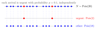
In the figure, $N\sim\operatorname{Pois}(20)$ arrivals are each marked urgent with probability $p=0.1$ $0.1$ , independently. The urgent arrivals form a $\operatorname{Pois}(2)$ count and the others a $\operatorname{Pois}(18)$ count; in this sample there are $2$ urgent and $18$ other arrivals. By independence, knowing how many urgent arrivals occurred says nothing about the number of other arrivals.

This is the chicken–egg theorem phrased in terms of labels, and both of its conditions matter. The labels must be independent of each other and of $N$ . The total must also be Poisson: for a fixed total $n$ , the type-1 count is $\operatorname{Bin}(n,p)$ and the type-2 count is $n$ minus it, so the two are dependent when $n\ge1$ and $0<p<1$ $1$ . If $n=0$ or $p\in\{0,1\}$ ${0, 1}$ , both counts are deterministic and independent. With a random total of another distribution they are in general dependent as well.

A common misreading is that the type-1 count is binomial and therefore tied to the type-2 count. It is binomial only conditionally on $N=n$ $n$ ; averaged over the Poisson total it is $\operatorname{Pois}(\lambda p)$ and independent of the other count. Splitting reverses Poisson merging, which adds the two counts back into $N$ . For a fixed number of items, the counts of several label types follow the multinomial distribution instead, and distinct category counts with positive probabilities are dependent when the total is positive.

Key Results¶

The two parameters add to the original parameter: $\lambda p+\lambda(1-p)=\lambda$ $λ$ .
For $k$ independent categorical labels with probabilities $p_i$ , the category counts are independent $\operatorname{Pois}(\lambda p_i)$ variables.

Examples¶

A Poisson arrival count of mean $20$ , labelled urgent with probability $0.1$ , yields independent counts of means $2$ and $18$ .
For mean $12$ and label probabilities $1/6,1/3,1/2$ , the three counts are independent Poisson variables of means $2,4,6$ .

Prerequisites¶

Chicken–Egg Theorem

Sources¶

Nicky van Foreest · Probability Distributions · Week 1

Aliases: Poisson thinning Symbols: element of, lambda

Last updated: 27 October 2026 11:52