Covariance¶

Definition¶

For square-integrable $X,Y$ , covariance is

\operatorname{Cov}(X,Y)=\mathbb{E}[(X-\mathbb{E}X)(Y-\mathbb{E}Y)] =\mathbb{E}[XY]-\mathbb{E}X\,\mathbb{E}Y.

Independence implies zero covariance; the converse generally fails.

Expanding the product of centred variables and using Linearity of Expectation gives $\operatorname{Cov}(X,Y)=\mathbb{E}[XY]-\mathbb{E}X\,\mathbb{E}Y$ $E X E Y$ .

Interpretation¶

Covariance measures whether two variables tend to deviate from their means in the same direction: it is positive when large values of $X$ tend to go with large values of $Y$ , and negative when they tend to go with small values. It also accounts for dependence in the variance of a sum.

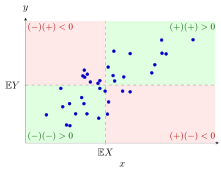
A scatter plot divided into four quadrants by lines at the means of X and Y; most points lie in the upper-right and lower-left quadrants, where the product of deviations is positive.

Points in the green quadrants contribute positive products of deviations, while points in the red quadrants contribute negative products. Covariance averages these products, taking both their magnitudes and probabilities into account.

The first formula in the Definition carries the meaning; the second, $\mathbb{E}[XY]-\mathbb{E}X\,\mathbb{E}Y$ $E X E Y$ , is the shortcut for computing, with $\mathbb{E}[XY]$ found from a joint PMF or density by two-dimensional LOTUS (continuous version). Taking $Y=X$ gives $\operatorname{Cov}(X,X)=\operatorname{Var}(X)$ $Var (X)$ . Shifts do not matter, but rescaling does: covariance carries the product of the units of $X$ and $Y$ , so only its sign is directly interpretable. Correlation divides by the standard deviations to remove the units.

In $\operatorname{Var}(X+Y)=\operatorname{Var}(X)+\operatorname{Var}(Y)+2\operatorname{Cov}(X,Y)$ $2 Cov (X, Y)$ , positive covariance means the deviations reinforce each other and negative covariance means they partly cancel. For independent variables the covariance is zero and the variances simply add, as in Probability Theory. Counts that compete for a fixed total have negative covariance, as in the multinomial distribution.

Zero covariance does not imply independence: for $X\sim\operatorname{Unif}(-1,1)$ and $Y=X^2$ $X^{2}$ , $\operatorname{Cov}(X,Y)=\mathbb{E}[X^3]-\mathbb{E}X\,\mathbb{E}[X^2]=0$ $0$ , although $Y$ is a function of $X$ .

Key Results¶

$\operatorname{Cov}(a+bX,c+dY)=bd\operatorname{Cov}(X,Y)$ $b d Cov (X, Y)$ .
$\operatorname{Var}(X+Y)=\operatorname{Var}(X)+\operatorname{Var}(Y)+2\operatorname{Cov}(X,Y)$ $2 Cov (X, Y)$ .

Examples¶

If $Y=2X$ and $\operatorname{Var}(X)=3$ $3$ , then $\operatorname{Cov}(X,Y)=6$ and $\operatorname{Var}(X+Y)=27$ $27$ .
For independent fair Bernoulli variables, $\mathbb{E}[XY]=1/4$ and $\mathbb{E}X\mathbb{E}Y=1/4$ $1/4$ , so covariance is zero.

Prerequisites¶

Sources¶

Nicky van Foreest · Probability Distributions · Week 2

Last updated: 22 October 2026 19:04