Weak Law of Large Numbers¶

Theorem¶

Let $X_1,X_2,\ldots$ be independent and identically distributed, with $\mathbb{E}|X_1|<\infty$ and mean $\mu$ . Then their sample mean satisfies

\bar X_n=\frac{1}{n}\sum_{i=1}^nX_i\xrightarrow{P}\mu.

Probability Distributions uses the sufficient finite-variance case $\operatorname{Var}(X_1)=\sigma^2<\infty$ $\infty$ , which admits the explicit Chebyshev proof below. Finite variance is not required for the more general integrable i.i.d. statement.

The conclusion is Convergence in Probability, so it asks whether each fixed-tolerance error probability tends to zero. In the finite-variance case, Chebyshev Inequality bounds that probability by $\sigma^2/(n\varepsilon^2)$ , which does tend to zero.

Interpretation¶

For a large i.i.d. sample with a finite mean, the sample mean is close to the population mean with high probability: for every fixed tolerance $\varepsilon>0$ $0$ , $\mathbb{P}(|\bar X_n-\mu|>\varepsilon)\to0$ $0$ . Finite variance additionally supplies a quantitative bound through the Chebyshev inequality.

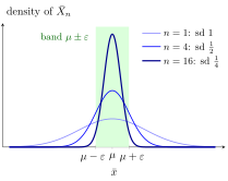
Densities of the sample mean for n = 1, 4 and 16, becoming narrower and taller around mu, with a shaded band from mu minus epsilon to mu plus epsilon.

The figure shows the normal example: for i.i.d. normal observations with standard deviation $\sigma=1$ $1$ , it plots the normal densities of $\bar X_n$ for $n=1$ $1$ , $4$ and $16$ . Other observation laws need not give these same density curves. Since $\operatorname{Var}(\bar X_n)=\sigma^2/n$ $σ^{2} / n$ , the standard deviation $\sigma/\sqrt n$ halves each time $n$ is multiplied by four: $1$ , $\tfrac{1}{2}$ , $\tfrac{1}{4}$ . The probability outside the band $\mu\pm\varepsilon$ therefore shrinks, and by Chebyshev it is at most $\sigma^2/(n\varepsilon^2)\to0$ $0$ .

The finite-variance proof uses two facts: $\mathbb{E}\bar X_n=\mu$ by linearity of expectation, and $\operatorname{Var}(\bar X_n)=\sigma^2/n$ $σ^{2} / n$ , because variances of independent terms add. Independence matters: if every $X_i$ equals $X_1$ , then $\bar X_n=X_1$ and its spread never shrinks. The bound also shows how the sample size must grow when the tolerance shrinks: halving $\varepsilon$ requires four times as many observations for the same bound.

The weak law does not generally assert that the absolute error $S_n-n\mu$ $n μ$ , where $S_n=n\bar X_n$ $n \overset{ˉ}{X}_{n}$ , tends to zero. For positive finite variance, that error has standard deviation $\sigma\sqrt n$ , which grows, while the average's standard deviation shrinks. In the degenerate case $\sigma=0$ $0$ , every observation equals $\mu$ almost surely and $S_n=n\mu$ exactly. The central limit theorem describes the size and shape of the remaining error $\bar X_n-\mu$ on the scale $\sigma/\sqrt n$ , and the strong law strengthens the conclusion to almost-sure convergence.

Key Results¶

$\operatorname{Var}(\bar X_n)=\sigma^2/n$ $σ^{2} / n$ .
Chebyshev gives $\mathbb{P}(|\bar X_n-\mu|\ge\varepsilon)\le\sigma^2/(n\varepsilon^2)\to0$ for each $\varepsilon>0$ $0$ .

Examples¶

For i.i.d. $\operatorname{Bern}(0.4)$ variables, the proportion of successes converges in probability to $0.4$ .
For i.i.d. $\operatorname{Exp}(2)$ variables and $n=1000$ $1000$ , the probability that the sample mean differs from $0.5$ by at least $0.1$ is at most $0.25/(1000(0.1)^2)=0.025$ $0.025$ .

Prerequisites¶

Sources¶

Nicky van Foreest · Probability Distributions · Week 7

Aliases: WLLN, weak law Symbols: epsilon, infinity, mu, sigma, square root, sum

Last updated: 27 October 2026 11:52