Density of an Order Statistic¶

Theorem¶

Let $X_1,\dots,X_n$ be i.i.d. continuous random variables with PDF $f$ and CDF $F$ , let $X_{(1)}\le\cdots\le X_{(n)}$ be their order statistics, and write $\bar F=1-F$ $F$ . For $1\le k\le n$ $n$ , the $k$ th order statistic has density

f_{X_{(k)}}(x)= n f(x) {\binom{n-1}{k -1}} \times F(x)^{k-1} \bar F(x)^{n-k}.

The formula holds for every $x$ except possibly on a set of zero length, for example at finitely many points.

The i.i.d. assumption makes the probabilities of falling below a threshold equal and independent. It produces the binomial count underlying the order-statistic CDF and density.

Interpretation¶

An order statistic is a sorted observation. Its density combines the chance of an observation near a value with the chances that the required numbers of observations fall below and above it.

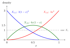
Densities of the minimum, median and maximum of three uniform observations on 0 to 1, peaking at 0, in the middle and at 1, with the flat density of one observation for comparison.

For three i.i.d. $\operatorname{Unif}(0,1)$ observations, the $k$ th order statistic has density $f_{X_{(k)}}(x)=3\binom{2}{k-1}x^{k-1}(1-x)^{3-k}$ for $0<x<1$ and $k=1,2,3$ $1, 2, 3$ : the minimum $3(1-x)^2$ peaks at $0$ , the median $6x(1-x)$ peaks at $1/2$ and the maximum $3x^2$ peaks at $1$ . The dashed line is the density of a single observation.

For $X_{(k)}$ to lie in a short interval of length $\Delta x$ at $x$ , one of the $n$ observations must lie there (factor $n$ , probability about $f(x)\Delta x$ ), and of the remaining $n-1$ $1$ , exactly $k-1$ must fall below $x$ . That count is binomial with $n-1$ trials and success probability $F(x)$ , which gives $\binom{n-1}{k-1}F(x)^{k-1}\bar F(x)^{n-k}$ . The i.i.d. assumption gives every observation the same probability $F(x)$ and makes the trials independent. Continuity makes exact ties have probability zero, but several observations can still fall in the same short interval. At a point where $f$ is continuous and finite, the probability of two or more observations in that interval is of order $(\Delta x)^2$ , so the one-observation calculation gives the first-order term used for the density. For discrete observations ties occur and the formula does not apply.

For $k=n$ and $k=1$ the formula is the derivative of the CDFs $F(x)^n$ and $1-\bar F(x)^n$ from Order Statistic, with $\bar F$ the survivor function.

The factor $n$ is easy to forget. Without it the density of the maximum of three uniforms would be $x^2$ , which integrates to $1/3$ instead of $1$ .

Key Results¶

For the maximum, $F_{X_{(n)}}(x)=F(x)^n$ and $f_{X_{(n)}}(x)=nf(x)F(x)^{n-1}$ $n f (x) F (x)^{n - 1}$ .
For the minimum, $F_{X_{(1)}}(x)=1-(1-F(x))^n$ and $f_{X_{(1)}}(x)=nf(x)(1-F(x))^{n-1}$ $F (x))^{n - 1}$ .

Examples¶

For the maximum of three i.i.d. $\operatorname{Unif}(0,1)$ variables, the density is $3x^2$ on $(0,1)$ and $\mathbb{P}(X_{(3)}\le1/2)=1/8$ $1/8$ .
The minimum of four independent $\operatorname{Exp}(2)$ variables has tail $\mathrm{e}^{-8x}$ for $x\ge0$ $0$ , hence distribution $\operatorname{Exp}(8)$ .

Prerequisites¶

Sources¶

Nicky van Foreest · Probability Distributions · Week 3

Symbols: delta

Last updated: 27 October 2026 11:52