Continuous Bayes Rule¶

Theorem¶

For continuous random variables $X$ and $Y$ and an observed value $x$ with $0<f_X(x)<\infty$ $\infty$ ,

\begin{aligned} f_{Y\mid X}(y\mid x)=\frac{f_{X\mid Y}(x\mid y)\,f_Y(y)}{f_X(x)}. \end{aligned}

Equalities between conditional densities may fail on a set of zero length, for example at finitely many points.

The Continuous Law of Total Probability computes the normalizing marginal density by averaging the likelihood against the conditioning variable’s density. That normalizer makes the reversed conditional density integrate to one.

Interpretation¶

Bayes’ rule for densities turns a model of how the observation depends on the unknown into a statement about the unknown. The likelihood $f_{X\mid Y}(x\mid y)$ times the prior density $f_Y(y)$ , normalized by the marginal density $f_X(x)$ of the observation, gives the posterior density $f_{Y\mid X}(y\mid x)$ $x)$ .

Prior density 2y, likelihood 1/y and the resulting posterior, which is flat at 5/3 on the interval from 0.4 to 1 after observing X = 0.4.

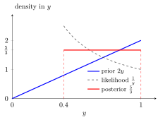
The illustrated joint density equals $2$ on $0<x<y<1$ $1$ . For the observation $X=0.4$ $0.4$ , the prior density $f_Y(y)=2y$ and the likelihood $f_{X\mid Y}(0.4\mid y)=1/y$ for $0.4<y<1$ have the constant product $2$ ; dividing by $f_X(0.4)=2(1-0.4)=1.2$ gives the flat red posterior of height $5/3$ . The posterior is uniform on $(0.4,1)$ , in line with the first Example.

Read the formula with $x$ fixed. The denominator $f_X(x)$ does not depend on $y$ : it is only the constant that makes the posterior integrate to one, computed by the continuous law of total probability, so one may find the shape first and normalize at the end. The condition $0<f_X(x)<\infty$ replaces the discrete requirement that the observed event has positive probability: $\{X=x\}$ itself has probability zero, so a ratio of densities replaces a ratio of probabilities.

It is the discrete rule from Probability Theory with probabilities replaced by densities; the mixed discrete and continuous versions are on Bayes and Total Probability: Four Forms.

The posterior is a density in $y$ , but the likelihood $f_{X\mid Y}(x\mid y)$ $y)$ , read as a function of $y$ , need not be one: in the figure, $\int_{0.4}^1(1/y)\,\mathrm{d}y=\ln2.5\approx0.92$ $0.92$ , not $1$ .

Key Results¶

The normalizing density is $f_X(x)=\int f_{X\mid Y}(x\mid y)f_Y(y)\,\mathrm{d}y$ $y) f_{Y} (y) d y$ .
For fixed $x$ , $f_{Y\mid X}(y\mid x)$ is proportional in $y$ to likelihood times prior.

Examples¶

For density $2$ on $0<x<y<1$ $1$ , $f_{Y\mid X}(y\mid x)=1/(1-x)$ on $x<y<1$ $1$ .
For independent $X,Y\sim\operatorname{Unif}(0,1)$ $Unif (0, 1)$ , likelihood and marginal cancel, so the posterior density of $Y$ remains $1$ on $(0,1)$ .

Prerequisites¶

Sources¶

Nicky van Foreest · Probability Distributions · Week 2

Aliases: Bayes' rule for densities, Bayes' theorem for densities Symbols: infinity, integral

Last updated: 20 October 2026 03:02