Location and Scale Property of the MGF¶

Proposition¶

For real constants $a$ and $b$ (no positivity is needed for $b$ ),

\begin{aligned} M_{a+bX}(t)=\mathrm{e}^{a t}M_X(b t) \end{aligned}

for every $t$ at which $M_X(bt)$ is finite.

Starting from the Moment Generating Function definition, $\mathbb{E}[\mathrm{e}^{t(a+bX)}]=\mathrm{e}^{at}\mathbb{E}[\mathrm{e}^{(bt)X}]$ $e^{a t} E [e^{(b t) X}]$ . The deterministic shift comes outside the expectation and the scale changes the MGF argument.

Interpretation¶

A shift contributes an exponential factor to an MGF, while a scale changes its argument. Both follow from $\mathrm{e}^{t(a+bX)}=\mathrm{e}^{at}\,\mathrm{e}^{(bt)X}$ $e^{a t} e^{(b t) X}$ : the constant factor $\mathrm{e}^{at}$ moves outside the expectation, and the scale $b$ stays inside, where it multiplies $t$ .

A standard normal density and the density of 5 + 2Z, shifted right to mean 5 and spread wider by a factor 2, with an arrow labelled times 2, then plus 5.

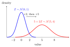
The figure turns the standard normal $Z$ into $5+2Z$ $2 Z$ : the density is first spread wider by the factor $2$ and then shifted to centre $5$ . In MGF terms, $M_Z(t)=\mathrm{e}^{t^2/2}$ gives $M_{5+2Z}(t)=\mathrm{e}^{5t}M_Z(2t)=\mathrm{e}^{5t+2t^2}$ $e^{5 t + 2 t^{2}}$ . This is the MGF $\mathrm{e}^{\mu t+\sigma^2t^2/2}$ of $\mathcal{N}(\mu,\sigma^2)$ with $\mu=5$ and $\sigma^2=4$ $4$ .

The expression $a+bX$ means scaling by $b$ first and shifting by $a$ second. Because the scale enters through $M_X(bt)$ , the formula holds only where $M_X(bt)$ is finite: for $X\sim\operatorname{Exp}(1)$ $Exp (1)$ , $M_{2X}(t)=1/(1-2t)$ is finite only for $t<\tfrac{1}{2}$ $\frac{1}{2}$ . A negative $b$ reflects the distribution, and the formula covers that case without change.

Differentiating at $t=0$ recovers the familiar rules $\mathbb{E}[a+bX]=a+b\,\mathbb{E}X$ and $\operatorname{Var}(a+bX)=b^2\operatorname{Var}(X)$ $b^{2} Var (X)$ , as in moments from the MGF. Combined with uniqueness, the property shows that $a+bZ\sim\mathcal{N}(a,b^2)$ for every $b\neq0$ $0$ , which is the basis of standardization.

Key Results¶

The formula is valid where $M_X(bt)$ is finite.
For $b=0$ $0$ , $M_{a+bX}(t)=\mathrm{e}^{at}$ $e^{a t}$ , the MGF of the constant $a$ .

Examples¶

For $X\sim\operatorname{Bern}(p)$ $Bern (p)$ , $M_{2+3X}(t)=\mathrm{e}^{2t}(1-p+p\mathrm{e}^{3t})$ $p e^{3 t})$ .
For $Z\sim\mathcal{N}(0,1)$ $N (0, 1)$ , $M_{5+2Z}(t)=\mathrm{e}^{5t+2t^2}$ $e^{5 t + 2 t^{2}}$ , so $5+2Z\sim\mathcal{N}(5,4)$ $N (5, 4)$ .

Prerequisites¶

Moment Generating Function

Sources¶

Nicky van Foreest · Probability Distributions · Week 1

Aliases: MGF of a linear transformation Symbols: mu, sigma

Last updated: 20 October 2026 03:02