Central Limit Theorem¶

Theorem¶

Let $X_1,X_2,\ldots$ be i.i.d. with mean $\mu$ and finite positive variance $0<\sigma^2<\infty$ $\infty$ . Then the sample mean $\displaystyle \bar X_n=\frac{1}{n}\sum_{i=1}^n X_i$ satisfies

\begin{aligned} \frac{\bar X_n-\mu}{\sigma/\sqrt{n}}\xrightarrow{d}\mathcal{N}(0,1). \end{aligned}

Equivalently, for the sum $\displaystyle S_n=\sum_{i=1}^n X_i$ $i = 1 \sum n X_{i}$ ,

\begin{aligned} \frac{S_n-n\mu}{\sigma\sqrt{n}}\xrightarrow{d}\mathcal{N}(0,1). \end{aligned}

Here $\mathcal{N}(\mu,v)$ denotes a normal distribution with mean $\mu$ and variance $v$ , and $\Phi$ is the standard normal CDF.

The i.i.d. assumption supplies the common distribution and independence used by the theorem. The arrow denotes Convergence in Distribution: the CDF of the standardized average tends to the standard normal CDF at each real threshold.

Interpretation¶

The properly centred and scaled fluctuations of an i.i.d. sum approach a standard normal distribution, whatever the distribution of the individual terms, provided their variance is finite and positive. This gives approximate probabilities for sums and averages that would be hard to compute exactly.

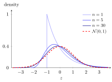
Densities of the standardized mean of n exponential observations for n = 1, 5 and 30, shifting from a strongly skewed shape towards the standard normal curve drawn for comparison.

The figure shows the density of $Z_n=(\bar X_n-\mu)/(\sigma/\sqrt n)$ for i.i.d. $\operatorname{Exp}(1)$ observations, so $\mu=\sigma=1$ $1$ , together with the standard normal density. For $n=1$ $1$ , $Z_1=X_1-1$ is an exponential density shifted to start at $-1$ , strongly skewed. For $n=5$ it is already a hump, and by $n=30$ it is close to the normal curve, with a slight remaining skew to the right. Since $n\bar X_n$ has a gamma distribution, these curves are rescaled gamma densities.

The scaling is essential. By the law of large numbers, $\bar X_n-\mu$ itself shrinks to $0$ ; dividing by the standard deviation $\sigma/\sqrt n$ of $\bar X_n$ is standardization, which keeps the variance at $1$ for every $n$ and makes the shape visible. The conclusion is convergence in distribution: the theorem gives probabilities $\mathbb{P}(Z_n\le z)\approx\Phi(z)$ $Φ (z)$ , not a statement about the values of $Z_n$ .

For Bernoulli terms the theorem becomes the normal approximation to the binomial, and for integer-valued sums the continuity correction improves it. A common misreading is that the observations themselves become normal for large $n$ . They keep their own distribution; only the standardized sum or average is approximately normal.

Key Results¶

For large $n$ , $S_n$ is approximately $\mathcal{N}(n\mu,n\sigma^2)$ and $\bar X_n$ approximately $\mathcal{N}(\mu,\sigma^2/n)$ .
The finite-sample approximation is not an exact normality claim; i.i.d. normal observations are a special case where the standardized sum is exactly normal.

Examples¶

For $100$ i.i.d. $\operatorname{Exp}(1)$ observations, $\mathbb{P}(\bar X_{100}\le1.1)\approx\Phi((1.1-1)/0.1)=\Phi(1)\approx0.8413$ $0.8413$ .
For $400$ independent fair die rolls, the sum has mean $1400$ and standard deviation $\sqrt{400(35/12)}\approx34.16$ $34.16$ ; $\mathbb{P}(S_{400}\le1434)$ is approximately $\Phi((1434.5-1400)/34.16)\approx0.8438$ with continuity correction.

Prerequisites¶

Sources¶

Nicky van Foreest · Probability Distributions · Week 8

Aliases: CLT Symbols: infinity, mu, phi, sigma, square root, sum

Last updated: 20 October 2026 03:02