Expected Payoff Maximization¶

Definition¶

In a decision problem under uncertainty, each action $a\in A$ induces a probability distribution (a lottery) over the outcome set $X$, and the decision maker has a payoff $v(x)$ for each outcome $x\in X$$X$.

• If $X=\{x_1,\ldots,x_m\}$ is finite, action $a$ gives outcome $x_k$ with probability $p(x_k\mid a)\ge0$$0$, where $\displaystyle \sum_{k}p(x_k\mid a)=1$$1$.
• If outcomes are continuous, action $a$ induces a density $f(x\mid a)$$a)$.

Assume each action has a finite expected absolute payoff; in the continuous case this means $\int_{-\infty}^{\infty}|v(x)|f(x\mid a)\,\mathrm{d}x<\infty$$\infty$. The expected payoff of action $a$ is

and expected payoff maximization means choosing $a^*\in\arg\max_{a\in A}\mathbb{E}[v(x)\mid a]$$a]$. A rational agent facing uncertainty is assumed to behave in this way.

Interpretation¶

The action does not fix the outcome; it changes the distribution of outcomes. The decision maker compares actions through the expectation of the payoff, computed from the probability mass function $p(\cdot\mid a)$ or the probability density function $f(\cdot\mid a)$$a)$. Computing $\mathbb{E}[v(x)\mid a]$ from the distribution of $x$, without first finding the distribution of $v(x)$, is LOTUS, in the discrete and the continuous case alike.

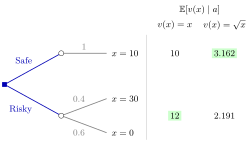
The figure draws Example 1. Each action leads to a chance node, that is, to a lottery over outcomes: Safe gives $x=10$ with probability $1$, Risky gives $30$ or $0$ with probabilities $0.4$ and $0.6$. The columns on the right are $\mathbb{E}[v(x)\mid a]$ for two payoff functions, with the larger value in each column shaded: with $v(x)=x$ Risky is chosen ($12>$$12>10$$10$), with $v(x)=\sqrt x$ Safe is chosen ($3.162>$$3.162>2.191$$2.191$).

Here the payoff values are cardinal: differences between payoffs matter, not only their order. A common misunderstanding is that the rule means maximizing expected money. That holds only when $v(x)=x$$x$. If $v$ is a strictly concave utility of money, the same rule is maximization of expected utility and describes a risk-averse decision maker (see expected utility and risk aversion).

In games, the uncertainty often comes from the other players: a belief about their choices plays the role of $p(\cdot\mid a)$$a)$, and from Week 2 a mixed strategy creates such uncertainty deliberately.

Key Results¶

• The expected payoff is linear in the probabilities: for a compound lottery that runs lottery $L_1$ with probability $\lambda$ and $L_2$ with probability $1-\lambda$$\lambda$, the expected payoff is $\lambda\,\mathbb{E}_{L_1}[v]+(1-\lambda)\,\mathbb{E}_{L_2}[v]$$\lambda ){\mathbb{E}}_{L_2}[v]$.
• Replacing $v$ by $\alpha v+\beta$ with $\alpha>0$ leaves the ranking of actions unchanged; a nonlinear strictly increasing transformation can reverse it (Example 1).
• If $A$ is finite and nonempty, a maximizing action exists under the finite-expected-payoff assumption above.
• With finitely many outcomes, the expected payoff of an action lies between the smallest and the largest payoff among the outcomes it can produce; in general it cannot exceed any upper bound, or fall below any lower bound, that holds for every payoff the action can produce.
• If every action leads to a single outcome with probability $1$, the rule reduces to choice under certainty.

Examples¶

1. Safe or risky. Action Safe pays $10$ for sure. Action Risky pays $30$ with probability $0.4$ and $0$ with probability $0.6$. With $v(x)=x$$x$,

so Risky is chosen. With $v(x)=\sqrt x$ instead, $\sqrt{10}\approx3.162$ against $0.4\sqrt{30}\approx2.191$$2.191$, so Safe is chosen: the ranking depends on the payoff scale, not only on the order of outcomes.

2. Continuous outcomes. Under action $a_1$ the outcome has the uniform distribution on $[0,20]$, so $f(x\mid a_1)=1/20$ and $\mathbb{E}[x\mid a_1]=10$$10$. Under $a_2$ the density is $f(x\mid a_2)=x/200$ on $[0,20]$ (it integrates to $400/400=1$$1$), so

With $v(x)=x$ the decision maker chooses $a_2$, which shifts probability towards high outcomes.

Prerequisites¶

• Rational Agent
• Expectation
• Probability Mass Function
• Probability Density Function

Related Concepts¶

• Expected Utility and Risk Aversion
• Mixed Strategy
• Best Response

Sources¶

• Game Theory · Week 1

Aliases: maximizing expected payoff, expected value criterion, Expected Payoff Maximisation Keywords: decision under uncertainty, lottery, p(x|a), f(x|a), E[v(x)|a], risk neutral Symbols: alpha, beta, element of, infinity, integral, lambda, square root, sum

Last updated: 27 October 2026 11:52