Cournot Duopoly¶

Definition¶

In a Cournot duopoly two firms produce a homogeneous good and simultaneously choose quantities $q_1,q_2\ge0$ $0$ . In the standard linear version:

the market price is given by the inverse demand $P(q_1+q_2)=\max\{a-b(q_1+q_2),\,0\}$ with $a>0$ $0$ , $b>0$ $0$ ;
each firm has constant marginal cost $c$ with $0\le c<a$ $a$ , so its cost is $c\,q_i$ ;
firm $i$ 's payoff is its profit $v_i(q_1,q_2)=\big(P(q_1+q_2)-c\big)q_i$ $c) q_{i}$ .

This is a static game of complete information with strategy sets $S_i=[0,\infty)$ $[0, \infty)$ .

Interpretation¶

Each firm's profit depends on the rival's quantity through the common price: more output by the rival lowers the price and makes one's own output less valuable. With positive marginal cost, a firm's best response is nonincreasing as the rival's quantity rises. Zero marginal cost has an additional boundary case described below.

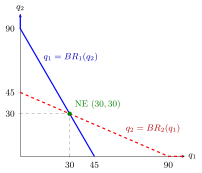
Reaction lines of the numerical Cournot example in the (q1, q2) plane: firm 1's best response runs from (0,90) to (45,0), firm 2's from (0,45) to (90,0), with zero-output branches beyond rival quantity 90 and crossing at (30,30).

The figure uses the numbers below ( $a =$ $a=100$ $100$ , $b=1$ $1$ , $c=10$ $10$ ). Firm 1's reaction line $q_1=\max\{(90-q_2)/2,0\}$ gives its profit-maximizing output for each $q_2$ , and firm 2's line $q_2=\max\{(90-q_1)/2,0\}$ does the same with the roles swapped. The positive-output portions slope downwards; when the rival produces at least $90$ , the best output is zero. The only point on both lines is $(30,30)$ , where each quantity is a best response to the other, so it is the Nash equilibrium.

The equilibrium is found by computing both best responses and solving them together, which is the definition of a Nash equilibrium applied to continuous strategies. Taking the partial derivative of $v_i$ with respect to the firm's own quantity, holding the rival's fixed, is the key step; differentiating the sum or the rival's quantity is a common error.

The positive-price equilibrium lies between monopoly and perfect competition: the firms together produce more than a monopolist, but less than the competitive output at which price equals marginal cost.

Key Results¶

For $0<c<a$ $a$ , the unique best response is the following. In the positive-price region, the first-order condition is $a-c-2bq_i-bq_j=0$ $0$ , with $\partial^2v_i/\partial q_i^2=-2b<0$ $0$ ; the nonnegative constraint gives the zero branch:

BR_i(q_j)=\max\Big\{\frac{a-c-bq_j}{2b},\,0\Big\}.

For $0<c<a$ $a$ , the unique Nash equilibrium is $q_1^*=q_2^*=\dfrac{a-c}{3b}$ $\frac{a - c}{3 b}$ , total output $Q^*=\dfrac{2(a-c)}{3b}$ $\frac{2 ( a - c )}{3 b}$ , price $P^*=\dfrac{a+2c}{3}$ $\frac{a + 2 c}{3}$ , profit $\dfrac{(a-c)^2}{9b}$ per firm.
At $c=0$ $0$ , the same positive-price equilibrium exists, but uniqueness fails under the stated truncated demand. If $q_j<a/b$ $a / b$ , the unique best response is $(a-bq_j)/(2b)$ $b q_{j}) / (2 b)$ ; if $q_j\ge a/b$ $a / b$ , every $q_i\ge0$ gives price zero and profit zero, so every quantity is a best response. Thus, in addition to the positive-price equilibrium, every profile with $q_1,q_2\ge a/b$ is a zero-price equilibrium.
A monopolist would produce $Q^m=\dfrac{a-c}{2b}$ $\frac{a - c}{2 b}$ ; perfect competition gives $Q^c=\dfrac{a-c}{b}$ $\frac{a - c}{b}$ ; so $Q^m<Q^*<Q^c$ $Q^{c}$ .
If each firm produced $\dfrac{a-c}{4b}$ (half the monopoly output), each would earn $\dfrac{(a-c)^2}{8b}>\dfrac{(a-c)^2}{9b}$ $\frac{( a - c ) ^{2}}{9 b}$ , but this is not an equilibrium: each firm's best response to $\dfrac{a-c}{4b}$ is $\dfrac{3(a-c)}{8b}$ . The equilibrium is not Pareto efficient for the firms.
With $n$ identical firms, a symmetric positive-price equilibrium is $q_i^*=\dfrac{a-c}{(n+1)b}$ $\frac{a - c}{( n + 1 ) b}$ .

Examples¶

Numbers. Let $a=100$ $100$ , $b=1$ $1$ , $c=10$ $10$ , so $P=100-q_1-q_2$ when $q_1+q_2\le100$ and $P=0$ otherwise.

In the region $q_1+q_2\le100$ $100$ , profit is $v_1=(90-q_1-q_2)q_1$ $q_{2}) q_{1}$ ; the first-order condition $90-2q_1-q_2=0$ gives $BR_1(q_2)=(90-q_2)/2$ for $q_2\le90$ $90$ .
By symmetry $q_2=(90-q_1)/2$ $q_{1}) /2$ . Solving this system of linear equations: $q_1=(90-(90-q_1)/2)/2$ $q_{1}) /2) /2$ , so $4q_1=90+q_1$ and $q_1=30$ $30$ .
Hence $q_1^*=q_2^*=30=(100-10)/3$ $10) /3$ , $P^*=40$ $40$ , profit $30\cdot30=900$ each.
Check: against $q_2=30$ $30$ , producing $31$ gives $(29)(31)=899$ and producing $29$ gives $(31)(29)=899$ $899$ , both below $900$ .

Prerequisites¶

Sources¶

Game Theory · Week 1

Aliases: Cournot competition, Cournot model, quantity competition, Cournot game, quantity-setting duopoly Keywords: inverse demand p = a - b(q1 + q2), q_i = (a - c)/(3b), reaction function, Cournot-Nash equilibrium, collusion, Cournot oligopoly Symbols: infinity, partial

Last updated: 27 October 2026 11:52