Affine Map¶

Definition¶

Let $n,\,k \in\mathbb{N}^+$${\mathbb{N}}^{+}$. A function $\boldsymbol{f}\colon \mathbb{R}^n\to \mathbb{R}^k$ is an affine map (or affine transformation) if there are a $k\times n$ real matrix $\boldsymbol{A}$ and a vector $\boldsymbol{b}\in\mathbb{R}^k$ such that

A real-valued affine map $f\colon \mathbb{R}^n\to \mathbb{R}$ ($k=$$k=1$$1$) is an affine function:

An affine map is a linear map exactly when $\boldsymbol{b}=\boldsymbol{0}$$0$, that is, when $\boldsymbol{f}(\boldsymbol{0})=\boldsymbol{0}$$0$.

As a Function between Spaces, the map assigns one output vector to each input vector. The Vector Space operations make the expression $\boldsymbol{A}\boldsymbol{x}+\boldsymbol{b}$ meaningful: first apply the matrix, then add the translation vector.

Interpretation¶

An affine map is a linear map followed by a shift: if one argument is increased by $c$ units, the value changes by $c$ times a fixed vector, wherever the starting point is.

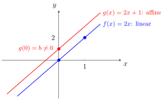
The blue linear map $f(x)=2x$ passes through the origin. The red affine map $g(x)=f(x)+1$ is shifted upwards by $1$, so $g(0)=1$ rather than $0$. Both lines have slope $2$: the matrix $\boldsymbol{A}$, here the number $2$, sets the slope, and $\boldsymbol{b}$ only moves the graph.

Both parts can be read off from $\boldsymbol{f}$: $\boldsymbol{b}=\boldsymbol{f}(\boldsymbol{0})$$\mathbf{f}(0)$, and $\boldsymbol{f}(\boldsymbol{x})-\boldsymbol{f}(\boldsymbol{y})=\boldsymbol{A}(\boldsymbol{x}-\boldsymbol{y})$$\mathbf{y})$, so a change in the output depends only on the change in the input. Affine maps keep affine combinations: $\boldsymbol{f}(\lambda\boldsymbol{x}+(1-\lambda)\boldsymbol{y})=\lambda\boldsymbol{f}(\boldsymbol{x})+(1-\lambda)\boldsymbol{f}(\boldsymbol{y})$ for every real $\lambda$. Hence they map lines to lines or points, and midpoints to midpoints. The image of $\mathbb{R}^n$ is the range of $\boldsymbol{x}\mapsto\boldsymbol{A}\boldsymbol{x}$$\mathbf{A}\mathbf{x}$, shifted by $\boldsymbol{b}$.

A common slip comes from the terminology in the note. $g(x)=2x+1$ is called a linear function in calculus, but it is not a linear map: $g(1+1)=5$$5$, while $g(1)+g(1)=6$$6$.

This idea returns later: a differentiable function of several variables is one that is approximated near a point by an affine map, just as a differentiable function of one variable is approximated by its tangent line.

Key Results¶

• The graph $\{(\boldsymbol{x},f(\boldsymbol{x}))\colon\boldsymbol{x}\in\mathbb{R}^n\}$ of an affine function on $\mathbb{R}^n$ is an affine hyperplane of $\mathbb{R}^{n+1}$; it passes through the origin exactly when $b=0\text{.}$
• The level sets $\{\boldsymbol{x}\colon f(\boldsymbol{x})=c\}$ of a non-constant affine function are parallel affine hyperplanes of $\mathbb{R}^n$.
• A composition of affine maps is affine.

Examples¶

• $f(x,y) = x + 2y - 1$ is affine but not linear, since $f(0,0)=-1$$-1$; $x+2y$ is both.
• $g(x,y) = x + xy$ and $h(x,y) = 2^x + \sin y$ are not affine.

Prerequisites¶

• Function between Spaces
• Linear Map
• Vector Space
• Matrix

Related Concepts¶

• Determinant
• Hyperplane
• Parametric Representations of Lines and Planes
• Plane

Sources¶

• Math III: Analysis · Lecture 7

Aliases: affine transformation Keywords: affine function, linear function (economics usage) Symbols: element of, lambda, natural numbers, real numbers

Last updated: 22 October 2026 19:04