Revenue Equivalence Theorem¶

Theorem¶

Suppose that

$n$ bidders are risk-neutral;
values are independent private values: $\theta_1,\dots,\theta_n$ are i.i.d. with a continuous cumulative distribution function (CDF) $F$ that has a positive density on $[\underline\theta,\overline\theta]$ , and each bidder knows only her own value;
two auction formats each have a Bayesian Nash equilibrium in which the object always goes to the bidder with the highest value;
in both equilibria a bidder with the lowest possible value $\underline\theta$ has expected surplus $0$ .

Then in both equilibria each type $\theta$ has the same expected payment

m(\theta)=\theta\,G(\theta)-\int_{\underline\theta}^{\theta}G(x)\,\mathrm{d}x,\qquad G(\theta)=F(\theta)^{n-1},

and the seller's expected revenue is the same, namely $\mathbb{E}[\theta_{(n-1)}]$ , the expectation of the second-highest value.

Interpretation¶

In equilibrium, a bidder's expected surplus $U(\theta)=\theta G(\theta)-m(\theta)$ is pinned down by two things only: the probability $G(\theta)$ of winning, which is fixed by the allocation rule (condition 3), and the surplus of the lowest type (condition 4). An envelope argument gives $U'(\theta)=G(\theta)$ $G (θ)$ , so $U(\theta)=U(\underline\theta)+\int_{\underline\theta}^\theta G(x)\,\mathrm{d}x$ $\int_{\underline{θ}}^{θ} G (x) d x$ . Expected payments, and so expected revenue, then cannot differ across formats.

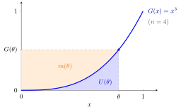
Curve G(x) = x³ for four bidders, with the rectangle θ·G(θ) split by the curve into the surplus U(θ) below it and the expected payment m(θ) above it.

The figure draws the payment formula for $n=4$ bidders with $\operatorname{Unif}(0,1)$ values, where $G(x)=x^3$ $x^{3}$ . A type- $\theta$ bidder wins with probability $G(\theta)$ , so the rectangle $\theta\,G(\theta)$ is the expected value of the object to her. The area under $G$ up to $\theta$ is her surplus $U(\theta)=\int_0^\theta G(x)\,\mathrm{d}x$ $\int_{0}^{θ} G (x) d x$ , and the rest of the rectangle, above the curve, is the expected payment $m(\theta)$ . Both areas depend only on $G$ , which the allocation rule fixes, and on the zero surplus of the lowest type, which is why the auction format drops out.

Move $\theta$ and $n$ : the area under $G$ is the surplus $U(\theta)$ and the rest of the rectangle is the expected payment $m(\theta)=\tfrac{n-1}{n}\theta^n$ $\frac{n - 1}{n} θ^{n}$ , whatever the auction format.

Each hypothesis matters. With risk-averse bidders the first-price auction yields more revenue than the second-price auction. With a reserve price above $\underline\theta$ , low types never win, so condition 3 fails and revenue can change. With asymmetric value distributions the first-price equilibrium need not allocate to the highest value. With affiliated or common values the formats can rank differently.

A common misunderstanding is that the formats give the same revenue in every realization. They do not: the theorem is about expected revenue. In a second-price auction the price is the realized second-highest value; in a first-price auction it is the winner's bid, which varies differently.

Key Results¶

With i.i.d. $\operatorname{Unif}(0,1)$ values, $G(\theta)=\theta^{n-1}$ and $m(\theta)=\frac{n-1}{n}\theta^n$ $\frac{n - 1}{n} θ^{n}$ ; expected revenue is $\mathbb{E}[\theta_{(n-1)}]=\frac{n-1}{n+1}$ $\frac{n - 1}{n + 1}$ , using the second-highest order statistic.
First-price, second-price, English, Dutch and all-pay auctions all satisfy the conditions in their symmetric equilibria with independent private values, so they are revenue-equivalent.
Each type's interim expected surplus is also equal across formats: $U(\theta)=\int_{\underline\theta}^\theta G(x)\,\mathrm{d}x$ $\int_{\underline{θ}}^{θ} G (x) d x$ , which is $\theta^n/n$ for $\operatorname{Unif}(0,1)$ .
The theorem can be used to find equilibrium bids: in a first-price auction a type- $\theta$ bidder pays $b(\theta)$ with probability $G(\theta)$ , so $b(\theta)=m(\theta)/G(\theta)$ $m (θ) / G (θ)$ .

Examples¶

Two bidders, $\operatorname{Unif}(0,1)$ . Here $G(\theta)=\theta$ and $m(\theta)=\theta^2-\theta^2/2=\theta^2/2$ $θ^{2} /2$ .

Second-price: the winner pays the rival's value; $\mathbb{E}[\min(\theta_1,\theta_2)]=\frac{1}{3}$ $\frac{1}{3}$ .
First-price: bids $\theta/2$ ; revenue $\frac{1}{2}\mathbb{E}[\max(\theta_1,\theta_2)]=\frac{1}{2}\cdot\frac{2}{3}=\frac{1}{3}$ $\frac{1}{3}$ .
All-pay (everyone pays her bid): the symmetric equilibrium bid equals $m(\theta)=\theta^2/2$ $θ^{2} /2$ , paid by both bidders; revenue $2\,\mathbb{E}[\theta^2/2]=2\cdot\frac{1}{6}=\frac{1}{3}$ $\frac{1}{3}$ .

Recovering a bid. For $n=4$ and $\operatorname{Unif}(0,1)$ values, $m(\theta)=\frac{3}{4}\theta^4$ and $G(\theta)=\theta^3$ $θ^{3}$ , so the first-price bid is $b(\theta)=\frac{3}{4}\theta$ and revenue is $\frac{3}{5}$ .

A violation. With $n=2$ $2$ , $\operatorname{Unif}(0,1)$ values and a reserve price $r=\frac{1}{2}$ in a second-price auction, the object is unsold when both values are below $\frac{1}{2}$ , so condition 3 fails. Expected revenue rises to $\frac{5}{12}>\frac{1}{3}$ $\frac{1}{3}$ .

Prerequisites¶

Sources¶

Game Theory · Week 6

Aliases: revenue equivalence, RET, revenue equivalence principle Keywords: expected revenue, expected second-highest value, all-pay auction, reserve price, lowest type zero surplus Symbols: integral, theta

Last updated: 22 October 2026 19:04