Bayes Rule for Beliefs¶

Method¶

Let $(\sigma,\mu)$ be an assessment: a strategy profile $\sigma$ and a system of beliefs $\mu$ . For an information set $h$ and a node $x\in h$ $h$ , write $\mathbb{P}_\sigma(x)$ for the probability that play reaches $x$ when Nature moves according to the common prior and players follow $\sigma$ . If $\displaystyle \mathbb{P}_\sigma(h)=\sum_{y\in h}\mathbb{P}_\sigma(y)>0$ $0$ , beliefs are consistent with Bayes' rule at $h$ when, for every $x\in h$ $h$ ,

\mu(x)=\frac{\mathbb{P}_\sigma(x)}{\sum_{y\in h}\mathbb{P}_\sigma(y)}.

Two types. Suppose an entrant is competitive ( $C$ ) with prior probability $p$ and weak ( $W$ ) with probability $1-p$ $p$ , and type $C$ enters with probability $q_C$ and type $W$ with probability $q_W$ . If $q_C\,p+q_W\,(1-p)>0$ $0$ , the incumbent's belief after observing entry is

\mu=\mathbb{P}(C\mid\text{entry}) =\frac{q_C\,p}{q_C\,p+q_W\,(1-p)}.

If $q_C\,p+q_W\,(1-p)=0$ $0$ , entry is off the equilibrium path and the formula places no restriction on $\mu$ .

Interpretation¶

This is Bayes' rule applied to the nodes of an information set: the prior over types is updated with the probability that each type takes the observed action. The denominator is the total probability of the observed action, by the law of total probability.

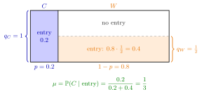
Area diagram of the mixed-strategy example: a strip for type C of width 0.2 fully shaded as entry, a strip for type W of width 0.8 half shaded, and the posterior 0.2/(0.2+0.4) = 1/3.

The figure draws the mixed-strategy example below. The widths of the two strips are the prior probabilities $p=0.2$ and $1-p=0.8$ $0.8$ , and the shaded height in each strip is that type's entry probability, $q_C=1$ and $q_W=\tfrac{1}{2}$ $\frac{1}{2}$ . Observing entry means play is somewhere in the shaded area, of total size $0.2+0.4=0.6$ $0.6$ ; the posterior $\mu$ is the share of that area belonging to type $C$ , namely $\tfrac{1}{3}$ .

Change $q_W$ : the posterior $\mu$ is type $C$ 's share of the shaded entry area. Set $q_C=q_W>0$ and it equals the prior; set $q_W=0$ with $q_Cp>0$ and it equals $1$ . If the total entry probability is zero, Bayes' rule does not determine the posterior.

The new element compared with Year-1 probability is that the "likelihoods" $q_C,q_W$ are not given by nature but chosen in equilibrium: they come from the players' strategies, possibly a mixed strategy. Beliefs and strategies are therefore determined jointly, and a change in one type's behaviour changes what the other side infers.

A common mistake is to apply the formula at an information set that is reached with probability zero, or to conclude that off-path beliefs must equal the prior. Neither is implied: Bayes' rule simply has nothing to say there.

Key Results¶

If all types take the observed action with the same probability ( $q_{C} =$ $q_C=q_W>0$ $0$ ), the posterior equals the prior: $\mu=p$ $p$ . This is the pooling case.
If only $C$ takes the action, with $q_W=0$ and $q_Cp>0$ $0$ , then $\mu=1$ $1$ ; if only $W$ takes it, with $q_C=0$ and $q_W(1-p)>0$ $0$ , then $\mu=0$ $0$ . The observed action then identifies its taker's type. This alone need not make the whole strategy profile separating: separation requires the types' equilibrium actions to distinguish them.
If the action is taken with probability $0$ by all types, $\mu$ is unrestricted by Bayes' rule.
For $0<p<1$ and a positive denominator, the posterior is nondecreasing in $q_C$ and nonincreasing in $q_W$ ; it is strictly monotone in both when $q_C>0$ and $q_W>0$ $0$ .
In a perfect Bayesian equilibrium, Bayes' rule is required at every information set reached with positive probability.

Examples¶

Pure strategies. Prior $p=\frac{1}{2}$ $\frac{1}{2}$ . If both types enter, $\mu=\frac{1\cdot0.5}{1\cdot0.5+1\cdot0.5}=0.5$ $0.5$ . If only $C$ enters, $\mu=\frac{0.5}{0.5+0}=1$ $1$ .

Mixed strategy. Prior $p=\frac{1}{5}$ $\frac{1}{5}$ . Type $C$ always enters ( $q_{C} =$ $q_C=1$ $1$ ) and type $W$ enters with probability $q_W=\frac{1}{2}$ $\frac{1}{2}$ . Then

\mu=\frac{1\cdot0.2}{1\cdot0.2+0.5\cdot0.8}=\frac{0.2}{0.6}=\frac{1}{3}.

Entry raises the probability of a competitive entrant from $0.2$ to $\frac{1}{3}$ , because type $W$ enters less often than type $C$ .

Inverse use. If the incumbent must hold belief $\mu=\frac{1}{3}$ after entry with $p=\frac{1}{5}$ and $q_C=1$ $1$ , the weak type's entry probability solves $\frac{0.2}{0.2+0.8\,q_W}=\frac{1}{3}$ $\frac{1}{3}$ , giving $q_W=\frac{2p}{1-p}=\frac{1}{2}$ $\frac{1}{2}$ .

Prerequisites¶

Sources¶

Game Theory · Week 7

Aliases: Bayesian updating of beliefs, Bayes' Rule for Beliefs, belief consistency Keywords: posterior belief, mu = q_C p / (q_C p + q_W (1-p)), on-path beliefs, zero-probability information set, Bayesian updating, entry game Symbols: element of, mu, sigma, sum

Last updated: 27 October 2026 11:52