Harsanyi Purification Theorem¶

Theorem¶

Informal statement (Harsanyi, 1973). Let $G$ be a finite normal-form game with payoffs $v_i(a)$, and let $\sigma^*$ be a Nash equilibrium in mixed strategies of $G$. For $\varepsilon>0$ consider the perturbed Bayesian game $G(\varepsilon)$ in which player $i$'s payoff is

where the perturbation vector $\theta_i=(\theta_i^a)_{a\in A}$ is player $i$'s privately observed type, drawn from a distribution with a continuous density, independently across players. Then, for generic $G$ (more precisely, for every regular equilibrium $\sigma^*$), there are equilibria of $G(\varepsilon)$ such that

• almost every type of every player has a unique best action, so the equilibrium is in pure strategies, and
• the probability with which each player's equilibrium strategy, viewed from outside, chooses each action converges to $\sigma_i^*$ as $\varepsilon\to0$$0$.

So every such mixed equilibrium is the limit of pure-strategy Bayesian Nash equilibria of slightly perturbed games of incomplete information.

Interpretation¶

In a mixed equilibrium each player is indifferent between the actions she mixes over, so it is unclear why she would randomize with exactly the equilibrium probabilities. Purification answers: she need not randomize at all. Small private payoff differences break her indifference one way or the other; an opponent who does not observe them sees a player whose action is random, with probabilities that approach the mixed equilibrium.

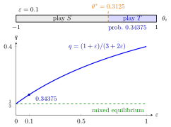
The figure uses the chicken game of the Examples. At the top, $\varepsilon=0.1$$0.1$: every type plays a pure action, $S$ below the cutoff $\theta^*=0.3125$ and $T$ above it, so an opponent who does not see $\theta_i$ observes $T$ with probability $(1-\theta^*)/2=0.34375$$0.34375$. Below, this probability $q=(1+\varepsilon)/(3+2\varepsilon)$ is plotted against $\varepsilon$; as the perturbation shrinks it falls to $\tfrac{1}{3}$, the probability of $T$ in the mixed equilibrium of the unperturbed game.

The limiting probabilities are pinned down by the opponents' incentives, not by the player's own. In the perturbed game, player $j$'s probability of an action must leave player $i$'s cutoff type exactly indifferent; as $\varepsilon\to0$ this forces it towards the value that makes $i$ indifferent in $G$, as in the indifference principle for mixed strategies.

The theorem is about limits of equilibria of nearby games, not about every perturbation of every game; nongeneric games can have mixed equilibria that cannot be purified.

Key Results¶

• Pure strategies in $G(\varepsilon)$ are type-contingent: typically a cutoff rule "choose action $x$ if and only if $\theta_i$ is above a threshold".
• The induced action distribution of player $i$ converges to $\sigma_i^*$ as $\varepsilon\to0$$0$.
• Pure Nash equilibria of $G$ that are strict are also approximated by equilibria of $G(\varepsilon)$, in which almost all types play the pure action.
• In the theorem the perturbations are private (each player observes only her own $\theta_i$) and independent across players; these are hypotheses, and the conclusion is not claimed without them.

Examples¶

The chicken game illustrates the construction. Actions are $S$ (swerve) and $T$ (go straight), with $v(S,S)=(0,0)$$(0,0)$, $v(S,T)=(-1,1)$$(-1,1)$, $v(T,S)=(1,-1)$$(1,-1)$, $v(T,T)=(-3,-3)$$(-3,-3)$. If the opponent plays $T$ with probability $q$, $S$ yields $-q$ and $T$ yields $1-4q$$4q$, so the symmetric mixed equilibrium has $q=\tfrac{1}{3}$$\frac{1}{3}$.

Perturbed game. Add $\varepsilon\theta_i$ to player $i$'s payoff from $T$, with $\theta_i$ having the uniform distribution on $[-1,1]$, independently and privately. Type $\theta_i$ prefers $T$ if and only if $1-4q+\varepsilon\theta_i\ge-q$$-q$, i.e. $\theta_i\ge\theta^*=(3q-1)/\varepsilon$$1)/\epsilon$. In a symmetric equilibrium $q=\mathbb{P}(\theta_j\ge\theta^*)=(1-\theta^*)/2$${\theta }^{\ast })/2$. Solving,

For $\varepsilon=0.1$$0.1$: $\theta^*=0.3125$ and $q=0.34375$$0.34375$. Every type plays a pure action (the cutoff type has probability 0), and $q\to\tfrac{1}{3}$ as $\varepsilon\to0$$0$.

Prerequisites¶

• Nash Equilibrium in Mixed Strategies
• Bayesian Nash Equilibrium
• Type
• Uniform Distribution

Related Concepts¶

• Chicken Game
• Indifference Principle for Mixed Strategies
• Harsanyi Transformation
• Mixed Strategy

Sources¶

• Game Theory · Week 5

Aliases: purification theorem, Harsanyi purification, purification of mixed equilibria Keywords: perturbed payoffs, payoff perturbations, private payoff shocks, interpretation of mixed strategies, cutoff strategy, epsilon to zero Symbols: element of, epsilon, sigma, theta

Last updated: 16 October 2026 22:28