Exponential Family¶

Definition¶

An exponential family is a family of probability laws whose mass function or density, relative to a fixed reference measure (counting for a probability mass function, so probabilities are sums; length for a probability density function, so probabilities are integrals), can be written as

f(y;\boldsymbol{\theta})=h(y)\exp\!\left\{\boldsymbol{\theta}^{\top}\boldsymbol{T}(y)-A(\boldsymbol{\theta})\right\}.

Here $\boldsymbol{\theta}$ is a vector of natural parameters, $\boldsymbol{T}(y)$ a vector of statistics, $(\cdot)^{\top}$ the transpose (written $(\cdot)^{\top}$ rather than the $(\cdot)^{\top}$ used on the other pages, to avoid a clash with the statistic $\boldsymbol{T}$ ), $h(y)$ a nonnegative base factor, and $A$ the log-normalizing function. The parameter domain contains values for which the normalizing sum or integral is finite. The support is fixed across the family in the regular setting used below.

For the one-parameter response families used in generalized linear models, the usual form is

f(y;\theta,\phi)=\exp\!\left\{\frac{y\theta-b(\theta)}{a(\phi)}+c(y,\phi)\right\}.

Here $\theta$ is the scalar natural parameter, $\phi$ a dispersion parameter, $a(\phi)>0$ a scale factor, $b$ the normalizing function, and $c$ the remaining term. This GLM form is a specialized representation; it does not describe every exponential family with an arbitrary statistic $\boldsymbol{T}(y)$ .

Interpretation¶

The mass function sums to one for a discrete response, whereas the density integrates to one for a continuous response. Their logarithms have the same parameter structure, allowing a common modelling framework for claim counts and continuous responses. An exponential family is a collection of distributions, not just the exponential waiting-time distribution.

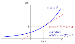
Graph of the Poisson normalizing function b(θ)=e^θ with its tangent at θ=log 2, where the slope b'(θ) equals the mean 2 and the curvature b''(θ) equals the variance 2.

The figure takes the Poisson row of the Examples table with $\lambda=2$ $2$ , so $\theta=\log 2$ and $b(\theta)=\mathrm{e}^\theta$ $e^{θ}$ . The slope of $b$ at that point is $b'(\theta)=2=\mu$ $μ$ , and its curvature is $b''(\theta)=2=\operatorname{Var}(Y)$ because $a(\phi)=1$ $1$ . Since $b$ is convex, the slope rises with $\theta$ , so a larger mean comes with a larger variance: the choice of family fixes this mean–variance relationship.

The expectation describes the response level and the variance its spread. In the GLM form, both follow from derivatives of $b$ , so choosing a response family also chooses a mean–variance relationship.

Key Results¶

When the support is parameter-independent and differentiation can pass through the normalizing sum or integral, the GLM form gives

\mu=\mathbb{E}[Y]=b'(\theta),\qquad \operatorname{Var}(Y)=a(\phi)b''(\theta).

For example, differentiating $\log f$ with respect to $\theta$ gives $(y-b'(\theta))/a(\phi)$ $b^{'} (θ)) / a (ϕ)$ . The derivative of the normalization condition has expectation zero, yielding the mean identity; differentiating again yields the variance identity. These calculations require the stated regularity, rather than just a visual resemblance to the formula.

The canonical link of a GLM is the link that makes the linear predictor the natural parameter, $g(\mu)=\theta$ $θ$ , that is $g=(b')^{-1}$ for the chosen representation. The response family and the link are separate choices; a GLM need not use its canonical link.

Examples¶

Response law	Natural parameter $\theta$	$b(\theta)$	$a(\phi)$	Mean and variance
Poisson, mean $\lambda>0$	$\log\lambda$	$\mathrm{e}^\theta$	$1$	Both equal $\lambda$
Bernoulli, $0<p<1$	$\log(p/(1-p))$	$\log(1+\mathrm{e}^\theta)$	$1$	$p$ and $p(1-p)$
Normal, mean $\mu$ , variance $\sigma^2>0$	$\mu$	$\theta^2/2$	$\sigma^2$	$\mu$ and $\sigma^2$

For the Poisson case, $c(y,\phi)=-\log(y!)$ for integer $y\ge0$ $0$ . This gives the log link and variance assumption used by Poisson regression. A count response with variance larger than its mean needs a different variance model; choosing a log link alone does not make its distribution Poisson.

Sources¶

CMU, Generalized Linear Models, exponential-family formulation.
Course placement: Risk Insurance, alongside the generalized linear model material; lecture assignment provisional (not checked against the course notes).

Prerequisites¶

Aliases: exponential family of distributions, exponential-family distribution Keywords: natural parameter, canonical link, mean b'(θ), variance a(φ) b''(θ), log-normalizing function, mean–variance relationship Symbols: lambda, mu, phi, sigma, theta

Last updated: 22 October 2026 19:04