Optimal Bonus-Malus Relativities¶

Proposition¶

For random claim rate $\Lambda$ and stationary class $L$, the unconstrained class value $r_l$ minimizing $\mathbb{E}[(\Lambda-r_L)^2]$ is $r_l=\mathbb{E}[\Lambda\mid L=l]$$l]$, for classes of positive probability and finite second moments. This is on a claim-frequency scale; dimensionless premium relativities require normalization by a base rate.

Interpretation¶

Each class is priced by the average underlying rate among its members. This minimizes squared prediction error, but can produce an irregular or commercially unsuitable scale.

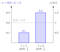
The figure draws the example below: two equally frequent classes whose members have average claim rates $\mathbb{E}[\Lambda\mid L=1]=0.1$ and $\mathbb{E}[\Lambda\mid L=2]=0.3$$0.3$. These are the optimal class values on the claim-frequency scale (left axis). Their probability-weighted average is $\tfrac{1}{2}(0.1)+\tfrac{1}{2}(0.3)=0.2=\mathbb{E}[\Lambda]$$\mathbb{E}[\Lambda ]$, in line with $\mathbb{E}[r_L]=\mathbb{E}[\Lambda]$$\mathbb{E}[\Lambda ]$; dividing by this base rate gives the dimensionless relativities $0.5$ and $1.5$ on the right axis.

The stationary bonus-malus distribution and premium supplies the long-run class probabilities used to weight claim rates within each class. Conditional expectation given a random variable minimizes squared prediction error within that class, giving $r_l=\mathbb{E}[\Lambda\mid L=l]$$l]$. Under a linear restriction, covariance measures the joint variation of risk and class, while variance and standard deviation supplies the class spread in the denominator of the regression slope.

Key Results¶

• If class probability at fixed rate is $\pi_l(\lambda)$ and rate density is $f_\Lambda$, then $r_l=\int\lambda\pi_l(\lambda)f_\Lambda(\lambda)\,\mathrm{d}\lambda/\int\pi_l(\lambda)f_\Lambda(\lambda)\,\mathrm{d}\lambda$$\int \lambda {\pi }_l(\lambda )f_{\Lambda }(\lambda )\mathrm{d}\lambda /\int {\pi }_l(\lambda )f_{\Lambda }(\lambda )\mathrm{d}\lambda$.
• $\mathbb{E}[r_L]=\mathbb{E}[\Lambda]$$\mathbb{E}[\Lambda ]$.
• Under a linear restriction $r_l=a+bl$ and $\operatorname{Var}(L)>0$$0$, $b=\operatorname{Cov}(\Lambda,L)/\operatorname{Var}(L)$ and $a=\mathbb{E}[\Lambda]-b\mathbb{E}[L]$$b\mathbb{E}[L]$.
• Refining the same information partition cannot increase unconstrained minimum mean squared error (MSE). Merely changing the number of classes in a different system does not guarantee an improvement.

Examples¶

If two equally frequent classes have conditional rates 0.1 and 0.3, their optimal frequency-scale values are 0.1 and 0.3. At base rate 0.2, the dimensionless relativities are 0.5 and 1.5.

Prerequisites¶

• Stationary Bonus-Malus Distribution and Premium
• Conditional Expectation Given a Random Variable
• Covariance
• Variance and Standard Deviation

Related Concepts¶

• Loimaranta Efficiency

Sources¶

• Risk Insurance · Lecture 14

Aliases: minimum-MSE BMS scale, linear premium relativities, optimal relativities, optimal premium relativities Keywords: r_l = E[Λ | L = l], mean squared error, b = Cov(Λ, L)/Var(L), normalization by a base rate Symbols: integral, lambda, pi

Last updated: 14 October 2026 08:21