Stationary Bonus-Malus Distribution and Premium¶

Definition¶

A stationary distribution at claim rate $\lambda$ , the general Markov-chain stationary distribution applied to the bonus-malus chain, is a row vector $\boldsymbol{\pi}(\lambda)$ satisfying $\boldsymbol{\pi} \boldsymbol{P}=\boldsymbol{\pi}$ $π$ , $\pi_l\ge0$ and $\displaystyle \sum_l\pi_l=1$ $1$ . With class premiums $c_l$ , the stationary mean premium is $\displaystyle b(\lambda)=\sum_l\pi_l(\lambda)c_l$ $l \sum π_{l} (λ) c_{l}$ .

Interpretation¶

The bonus-malus transition matrix advances the class probabilities by one year. Setting the output equal to the input gives a linear system for the stationary proportions, with a normalization equation ensuring that they sum to one. The stationary distribution leaves class proportions unchanged after another year. Convergence from arbitrary initial proportions is a separate property, not a consequence of solving the stationary equation alone.

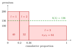
Rectangles for three bonus-malus classes, widths the stationary proportions 0.2, 0.16, 0.64 and heights the premiums 200, 200, 100; a dashed line marks the mean premium 136.

The figure uses the Examples numbers. Each class $l$ is a rectangle of width $\pi_l$ and height $c_l$ , so its area $\pi_lc_l$ is that class's contribution to the mean premium: $40+32+64=136$ $136$ . The dashed level $b(\lambda)=136$ is the single premium that would collect the same total from the stationary portfolio; it lies between the bonus premium 100 and the premium 200, closer to 100 because most of the stationary mass sits in the third class.

Key Results¶

A finite irreducible chain has a unique stationary distribution; aperiodicity additionally guarantees convergence from every initial distribution. These formal properties are covered in Year 3 Stochastic Models; solving the balance equations here does not require a convergence argument.
$\boldsymbol{\pi}$ is a left eigenvector of $\boldsymbol{P}$ for eigenvalue one, normalized to sum to one.
For the three-state two-year scheme, with $p=1-\mathrm{e}^{-\lambda}$ and $q=\mathrm{e}^{-\lambda}$ as in the transition-matrix example, $\boldsymbol{\pi}=(p,pq,q^2)$ $(p, pq, q^{2})$ .
If the first two states cost $c$ and the third costs $a$ , $b(\lambda)=c(1-\mathrm{e}^{-2\lambda})+a\mathrm{e}^{-2\lambda}$ $a e^{- 2 λ}$ .

Examples¶

With $p=0.2$ and $q=0.8$ $0.8$ , stationary proportions are $(0.2,0.16,0.64)$ . Premiums $(200,200,100)$ give mean premium $136$ .

Prerequisites¶

Sources¶

Risk Insurance · Lecture 13

Aliases: steady-state BMS premium, stationary rating-class distribution, stationary bonus-malus distribution, stationary BMS premium Keywords: πP = π, left eigenvector for eigenvalue one, b(λ) = Σ π_l c_l, balance equations, stationary mean premium Symbols: lambda, pi, sum

Last updated: 17 October 2026 21:53