Jacobian Matrix¶

Definition¶

Suppose $E\subseteq \mathbb{R}^n$ $R^{n}$ , and $\boldsymbol{x}_0$ is an interior point of $E$ . For a function $\boldsymbol{f}\colon E\to\mathbb{R}^k$ whose partial derivatives all exist at $\boldsymbol{x}=\boldsymbol{x}_0$ $x_{0}$ , the following $k\times n$ matrix

\begin{aligned} \boldsymbol{\mathrm{J}}\boldsymbol{f}(\boldsymbol{x}_0)&=\begin{pmatrix} \frac{\partial f_1}{\partial x_1}(\boldsymbol{x}_0) & \cdots & \frac{\partial f_1}{\partial x_n}(\boldsymbol{x}_0)\\[8pt] \vdots & \ddots & \vdots\\[4pt] \frac{\partial f_k}{\partial x_1}(\boldsymbol{x}_0) & \cdots & \frac{\partial f_k}{\partial x_n}(\boldsymbol{x}_0) \end{pmatrix}\\[10pt] &=\begin{pmatrix} \boldsymbol{\nabla} f_1 (\boldsymbol{x}_0)^{\top}\\ \vdots\\ \boldsymbol{\nabla} f_k (\boldsymbol{x}_0)^{\top} \end{pmatrix}\\[10pt] &=\left(\frac{\partial \boldsymbol{f}}{\partial x_1}(\boldsymbol{x}_0),\,\cdots,\,\frac{\partial \boldsymbol{f}}{\partial x_n}(\boldsymbol{x}_0)\right) \end{aligned}

is called the derivative matrix or the Jacobian matrix.

Each row is the Gradient of one scalar component $f_i$ . When the function is totally differentiable, multiplying this matrix by an increment gives the Linear Map that approximates the output change; the existence of partial derivatives alone does not guarantee that approximation.

Interpretation¶

The Jacobian matrix stacks all the partial derivatives of a vector-valued function, showing how each output changes with each input: the entry in row $i$ and column $j$ is $\partial f_i/\partial x_j$ . When $\boldsymbol{f}$ is totally differentiable, it is the matrix of the linear map that best approximates $\boldsymbol{f}$ near $\boldsymbol{x}_0$ .

An input square of side h and its affine approximation at f(x0); the output sides are h times the Jacobian columns, against the curved image grid.

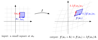
The square has sides $h\boldsymbol{e}_1$ and $h\boldsymbol{e}_2$ . Its image is approximated by the parallelogram with sides $h\,\mathrm{J}\boldsymbol{f}(\boldsymbol{x}_0)\boldsymbol{e}_1$ and $h\,\mathrm{J}\boldsymbol{f}(\boldsymbol{x}_0)\boldsymbol{e}_2$ . The figure uses $\boldsymbol{f}(u,v)=(1.3u+0.25v+0.08v^2,\,v+0.3u+0.1u^2)$ $0.1 u^{2})$ , $\boldsymbol{x}_0=(0.5,0.5)$ and $h=0.6$ $0.6$ . Thus $\boldsymbol{f}(\boldsymbol{x}_0)=(0.795,0.675)$ and the Jacobian columns are $(1.3,0.4)^{\top}$ and $(0.33,1)^{\top}$ . The filled output is the affine approximation, not the exact image under the nonlinear map; the curved grid shows the distinction.

Row $i$ is the transposed gradient of the component $f_i$ : how one output responds to all inputs. Column $j$ is $\partial\boldsymbol{f}/\partial x_j$ : how all outputs respond to one input. The matrix is $k\times n$ $n$ , outputs by inputs, so for $k=1$ it is the row vector $\boldsymbol{\nabla} f(\boldsymbol{x}_0)^{\top}$ , and for $n=k=1$ it is the $1\times1$ matrix $f'(x_0)$ .

For a totally differentiable $\boldsymbol{f}$ with $n=k$ $k$ , the absolute value of the determinant of the Jacobian is the factor by which $\boldsymbol{f}$ scales small areas or volumes near $\boldsymbol{x}_0$ , as $|\det\boldsymbol{A}|$ does for the linear map $\boldsymbol{h}\mapsto\boldsymbol{A}\boldsymbol{h}$ $A h$ . This factor appears in the transformation of densities of random vectors.

A common slip is to treat the Jacobian as the derivative whenever it exists. All partial derivatives can exist while $\boldsymbol{f}$ is not totally differentiable, and then the approximation above can fail. In Math IV, Jacobians return in the multivariable chain rule, where the matrices of composed functions are multiplied.

Key Results¶

The total derivative of a differentiable function is represented by the Jacobian matrix: the Jacobian is the matrix of this linear map with respect to the standard bases.
The existence of the Jacobian matrix does not necessarily imply the total differentiability of the function.

Examples¶

Let $\boldsymbol{f}(x,y) = (x^2, xy)$ $(x^{2}, x y)$ . Then $\dfrac{\partial \boldsymbol{f}}{\partial x} = (2x, y)$ $(2 x, y)$ , $\dfrac{\partial \boldsymbol{f}}{\partial y} = (0, x)$ $(0, x)$ , so

\boldsymbol{\mathrm{J}}\boldsymbol{f}(x,y) = \begin{pmatrix} 2x & 0 \\ y & x \end{pmatrix}.

Prerequisites¶

Total Derivative as a Linear Map

Sources¶

Math III: Analysis · Lecture 12

Aliases: Jacobian, derivative matrix, Jacobi matrix Symbols: nabla gradient, partial, real numbers, subset

Last updated: 27 October 2026 11:52