Homogeneous Function¶

Definition¶

Let $n,\,k \in\mathbb{N}^+$ and $m\in \mathbb{Z}$ $Z$ . A function $\boldsymbol{f}\colon \mathbb{R}^n\to \mathbb{R}^k$ is homogeneous of degree $m$ if

\boldsymbol{f}(cx_1,\dots,cx_n)=c^m \boldsymbol{f}(x_1,\dots,x_n)

for every $(x_1,\,x_2,\,\dots,\,x_n)$ and $c\neq 0$ $0$ . In economics one often uses the variant with domain $\mathbb{R}^n_{++}=(0,+\infty)^n$ $(0, + \infty)^{n}$ , only $c>0$ $0$ , and any real degree $m$ ; for example, $f(x,y)=x^{1/2}y^{1/2}$ is homogeneous of degree $1$ in this sense.

The definition treats $\boldsymbol{f}$ as a Function between Spaces: scaling an input vector changes its assigned output by the prescribed scalar factor.

Interpretation¶

If all arguments of a homogeneous function are multiplied by the same scalar $c$ , the value is multiplied by the fixed power $c^m$ of that scalar. The degree $m$ measures how strongly the function responds when all inputs are scaled together.

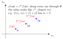
A ray from the origin with the points x, 2x and 3x, where the function takes the values f(x), 2 to the m times f(x) and 3 to the m times f(x).

Along the ray through $\boldsymbol{0}$ and $\boldsymbol{x}$ , the values are fixed by the single value $f(\boldsymbol{x})$ : at $2\boldsymbol{x}$ the function equals $2^mf(\boldsymbol{x})$ , and at $3\boldsymbol{x}$ it equals $3^mf(\boldsymbol{x})$ . For the figure's example $f(x_1,x_2)=x_1^2+x_2^2$ $x_{2}^{2}$ , with $m=2$ $2$ , these are $4f(\boldsymbol{x})$ and $9f(\boldsymbol{x})$ . Away from the origin, a homogeneous function is therefore determined by its values at one point of each ray.

The same factor $c$ must multiply every argument: scaling only $x_1$ says nothing about homogeneity. Degree $1$ means that doubling all inputs doubles the value, as for $x^{1/2}y^{1/2}$ ; in economics this is called constant returns to scale. Degree $0$ means $f(c\boldsymbol{x})=f(\boldsymbol{x})$ $f (x)$ , so only the ratios of the inputs matter, as for $x_1/x_2$ on $\mathbb{R}^2_{++}$ .

A linear map is homogeneous of degree $1$ , and a homogeneous polynomial of degree $k$ , such as a quadratic form, is homogeneous of degree $k$ .

A common slip is to add a constant: $x^2+y^2+1$ is not homogeneous, because the constant term does not scale with $c^2$ .

Key Results¶

If $f$ is homogeneous of degree $m$ and differentiable, then each partial derivative is homogeneous of degree $m-1$ $1$ .
The sum of two functions that are homogeneous of the same degree $m$ is homogeneous of degree $m\text{;}$ the product of scalar-valued functions homogeneous of degrees $m$ and $\ell$ is homogeneous of degree $m+\ell\text{,}$ and a well-defined composition of functions homogeneous of degrees $m$ and $p$ is homogeneous of degree $mp\text{.}$ A sum of two nonzero homogeneous functions of different degrees, such as $xy+x\text{,}$ is not homogeneous. The zero function is an exception to uniqueness of degree: it satisfies the homogeneity identity for every degree.

Examples¶

$f(x,y) = x^2 + y^2 + xy$ is homogeneous as $f(cx, cy) = c^2 f(x,y)$ $c^{2} f (x, y)$ .
$g(x,y) = xy + x$ is said to be inhomogeneous.

Prerequisites¶

Function between Spaces

Sources¶

Math III: Analysis · Lecture 7

Symbols: element of, infinity, integers, natural numbers, real numbers

Last updated: 27 October 2026 11:52