Saddle Point¶

Definition¶

Let $f\colon A\subseteq\mathbb{R}^n\to\mathbb{R}$ and let $\boldsymbol{a}\in A$$A$. The point $\boldsymbol{a}$ is a saddle point if it is a stationary point but is neither a local maximum nor a local minimum.

For a stationary point $\boldsymbol{a}$, this is equivalent to every neighbourhood containing points where $f$ is larger than $f(\boldsymbol{a})$ and points where $f$ is smaller than $f(\boldsymbol{a})$.

Interpretation¶

A saddle point is a flat-looking candidate where the function rises in some directions and falls in others: the tangent plane is horizontal, yet the point is no extremum.

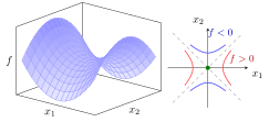
The figure shows $f(\boldsymbol{x})=x_1^2-x_2^2$ and its level curves. The level set $f=0$ consists of the two dashed lines $x_2=\pm x_1$$\pm x_1$, crossing at the origin: $f>0$ in the left and right sectors and $f<0$ in the upper and lower ones. At the origin $\boldsymbol{\nabla} f(\boldsymbol{0})=\boldsymbol{0}$ and $\boldsymbol{H}_f(\boldsymbol{0})=\operatorname{diag}(2,-2)$ is indefinite, so every neighbourhood contains both higher and lower values.

Negating the definitions of a local maximum and minimum gives an equivalent reading: a stationary point $\boldsymbol{a}$ is a saddle point exactly when every neighbourhood of $\boldsymbol{a}$ contains points where $f$ is larger than $f(\boldsymbol{a})$ and points where it is smaller. For $x_1^2-x_2^2$$x_2^2$, moving a distance $t$ in the direction at angle $\theta$ to the $x_1$-axis gives $f=t^2\cos2\theta$$t^2\cos 2\theta$, positive near the $x_1$-axis and negative near the $x_2$-axis. The function $xy$ from the Examples has the same shape turned by $45^\circ$, since $xy=\tfrac{1}{4}\big((x+y)^2-(x-y)^2\big)$$y{)}^2)$.

An indefinite Hessian at a stationary point guarantees a saddle (unconstrained extrema conditions), but a saddle does not need one: $x_1^4-x_2^4$ has a saddle at the origin with zero Hessian. A semidefinite Hessian does not decide between an extremum and a saddle: $x_1^2+x_2^4$ and $x_1^2-x_2^4$ both have Hessian $\operatorname{diag}(2,0)$ at the origin, the first has a minimum there and the second a saddle.

Key Results¶

• An indefinite Hessian at a critical point is the standard second-order signal for a saddle point.
• A zero gradient alone does not imply an extremum.
• Some saddle points require higher-order information because the Hessian test can be inconclusive.

Examples¶

• For $f(x,y)=x^2-y^2$$y^2$, $(0,0)$ is a saddle point because values increase along the $x$-axis and decrease along the $y$-axis.
• For $f(x,y)=xy$$xy$, $(0,0)$ is a saddle point because $xy$ takes positive and negative values arbitrarily close to the origin.

Prerequisites¶

• Critical Point
• Hessian Matrix

Related Concepts¶

• Local Maximum and Minimum on $\mathbb{R}^n$
• Unconstrained Extrema Conditions
• Hessian Test for Convexity and Concavity

Sources¶

• Math IV: Multivariate Calculus · Week 4, Lecture 1

Keywords: multivariable saddle Symbols: element of, nabla gradient, real numbers, subset, theta

Last updated: 27 October 2026 11:52