Method of Lagrange for Equality Constraints¶

Theorem¶

Let $A\subseteq\mathbb{R}^n$ be open. Consider

\begin{aligned} &\max_{\boldsymbol{x}\in A} f(\boldsymbol{x})\\ &\text{subject to}\quad h_j(\boldsymbol{x})=c_j,\ j=1,\ldots,m, \end{aligned}

with $C^1$ data and $m<n$ $n$ . Define

L(\boldsymbol{x},\boldsymbol{\mu})=f(\boldsymbol{x})+\sum_{j=1}^m\mu_j(c_j-h_j(\boldsymbol{x})).

If $f(\boldsymbol{x}^\ast)$ is a local maximum or minimum subject to the constraints, then either nondegenerate constraint qualification (NDCQ) fails at $\boldsymbol{x}^\ast$ or there exists $\boldsymbol{\mu}^\ast\in\mathbb{R}^m$ such that

\boldsymbol{\nabla} L(\boldsymbol{x}^\ast,\boldsymbol{\mu}^\ast)=0.

Interpretation¶

A regular equality-constrained optimum must be a critical point of the Lagrangian. The reason is that $f$ cannot be improved to first order by moving along the constraint set, which happens exactly when $\boldsymbol{\nabla} f$ is a linear combination of the constraint gradients.

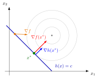
Circular level sets of f and the constraint line h(x) = c. At x star the gradients of f and h are parallel. At another point on the line they are not, so moving along the line still improves f.

The grey circles are level curves of $f$ around its unconstrained maximum, and the blue line is the constraint $h(\boldsymbol{x})=c$ $c$ . At $\boldsymbol{x}^\ast$ the level curve of the highest value that still meets the line just touches it, and the gradients of $f$ and $h$ are parallel: $\boldsymbol{\nabla} f(\boldsymbol{x}^\ast)=\mu\boldsymbol{\nabla} h(\boldsymbol{x}^\ast)$ $μ \nabla h (x^{*})$ . At the orange point $\boldsymbol{\nabla} f$ has a component along the line, so moving along $h(\boldsymbol{x})=c$ still increases $f$ .

The equations $\partial L/\partial x_i=0$ say $\displaystyle \boldsymbol{\nabla} f(\boldsymbol{x}^\ast)=\sum_j\mu_j^\ast\boldsymbol{\nabla} h_j(\boldsymbol{x}^\ast)$ $j \sum μ_{j}^{*} \nabla h_{j} (x^{*})$ , and $\partial L/\partial\mu_j=0$ gives back $h_j(\boldsymbol{x}^\ast)=c_j$ $c_{j}$ : $n+m$ equations for $n+m$ unknowns. NDCQ is needed for the multipliers to exist. Minimizing $x$ on the curve $x^3-y^2=0$ shows why: the minimizer is the origin, where $\boldsymbol{\nabla} h=(3x^2,-2y)$ is $\boldsymbol{0}$ , and no $\mu$ gives $(1,0)=\mu\boldsymbol{0}$ $μ 0$ . Such points are kept as separate candidates, and all candidates still have to be compared, since the conditions are only necessary.

The method optimizes the restriction of $f$ to the constraint set; without constraints it reduces to $\boldsymbol{\nabla} f=\boldsymbol{0}$ (unconstrained extrema conditions). The multiplier returns later as a shadow price: for $\max xy$ subject to $x+y=10$ from the Examples, the solution is $x=y=\mu^\ast=5$ $5$ ; with $10$ replaced by $c$ the best value $c^2/4$ grows at rate $c/2=5$ at $c=10$ $10$ .

Key Results¶

The theorem gives necessary, not sufficient, conditions.
Stationarity in the multiplier variables recovers the equality constraints.
Equality constraints can be written on either side because they have no direction.

Examples¶

Maximizing $xy$ subject to $x+y=10$ gives $L=xy+\mu(10-x-y)$ $y)$ .
Minimizing $x^2+y^2$ subject to $x+y=1$ uses the same equality-constrained stationarity method.

Prerequisites¶

Sources¶

Math IV: Multivariate Calculus · Week 4, Lecture 2

Keywords: Lagrange method with equalities, equality FONC, equality-constrained Lagrangian Symbols: element of, mu, nabla gradient, partial, real numbers, subset, sum

Last updated: 27 October 2026 11:52