Local Injectivity, Surjectivity, and Bijectivity¶

Theorem¶

Let $A\subseteq\mathbb{R}^n$${\mathbb{R}}^n$, let $\boldsymbol{f}\colon A\to\mathbb{R}^m$${\mathbb{R}}^m$, and let $\boldsymbol{x}_0\in\operatorname{int}(A)$ with $\boldsymbol{b}_0=\boldsymbol{f}(\boldsymbol{x}_0)$$\mathbf{f}({\mathbf{x}}_0)$.

• $\boldsymbol{f}$ is locally injective at $\boldsymbol{x}_0$ if there is an input neighbourhood $U\subseteq A$ of $\boldsymbol{x}_0$ on which $\boldsymbol{f}$ is injective. Equivalently, for every $\boldsymbol{b}\in\mathbb{R}^m$${\mathbb{R}}^m$, the equation $\boldsymbol{f}(\boldsymbol{x})=\boldsymbol{b}$ has at most one solution in $U$.
• $\boldsymbol{f}$ is locally surjective at $\boldsymbol{x}_0$ if nearby equations $\boldsymbol{f}(\boldsymbol{x})=\boldsymbol{b}$ have at least one nearby solution.
• $\boldsymbol{f}$ is locally bijective at $\boldsymbol{x}_0$ if nearby equations $\boldsymbol{f}(\boldsymbol{x})=\boldsymbol{b}$ have exactly one nearby solution.

If $\boldsymbol{f}$ is $C^1$, then (see the Jacobian rank theorem) full column rank of $\boldsymbol{D}\boldsymbol{f}(\boldsymbol{x}_0)$ implies local injectivity, full row rank implies local surjectivity, and square full rank implies local bijectivity.

Interpretation¶

These local properties study solutions of $\boldsymbol{f}(\boldsymbol{x})=\boldsymbol{b}$ near $\boldsymbol{x}_0$. Local injectivity requires a neighbourhood on which no two inputs have the same output, including outputs outside a chosen neighbourhood of $\boldsymbol{b}_0$. Local surjectivity and bijectivity concern existence and uniqueness of nearby solutions for nearby target values. In the $C^1$ applications below, continuity ensures that inputs sufficiently close to $\boldsymbol{x}_0$ also have outputs close to $\boldsymbol{b}_0$.

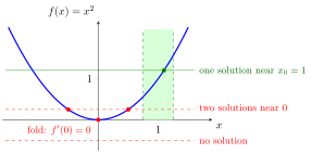
The function $f(x)=x^2$ is locally bijective near $x_0=1$$1$, where $f'(1)=2\neq0$$0$: inside the green band the line at height $1.2$ meets the graph once, at $x=\sqrt{1.2}\approx1.10$$1.10$. At the fold $x_0=0$$0$, where $f'(0)=0$$0$, the level $0.25$ has two preimages $\pm0.5$ close to $0$ and the level $-0.5$ has none, so $f$ is neither locally injective nor locally surjective there.

The rank conditions transfer facts about linear maps to $\boldsymbol{f}$. The linear map $\boldsymbol{h}\mapsto\boldsymbol{D}\boldsymbol{f}(\boldsymbol{x}_0)\boldsymbol{h}$ is injective if and only if its kernel is $\{\boldsymbol{0}\}$, which means full column rank, and surjective if and only if its range is all of $\mathbb{R}^m$, which means full row rank. By the Jacobian rank theorem, a $C^1$ map inherits the property of its Jacobian near $\boldsymbol{x}_0$. The rank conditions are sufficient, not necessary: $f(x)=x^3$ is bijective although $f'(0)=0$$0$.

Injectivity goes with a left inverse and surjectivity with a right inverse (left and right inverses). The square case $n=m$ is the multivariable inverse function theorem.

A common slip is to conclude a global property from local ones. The map $(x,y)\mapsto(\mathrm{e}^x\cos y,\mathrm{e}^x\sin y)$ has Jacobian determinant $\mathrm{e}^{2x}\neq0$$0$, so it is locally bijective at every point, yet $(x,y)$ and $(x,y+2\pi)$ have the same image.

Key Results¶

• Full column rank gives local uniqueness of nearby solutions.
• Full row rank gives local existence of nearby solutions.
• If $n=m$ and $\det(\boldsymbol{D}\boldsymbol{f}(\boldsymbol{x}_0))\neq0$$0$, the function is locally bijective at $\boldsymbol{x}_0$.

Examples¶

• The map $f(x,y)=x$ is locally surjective from $\mathbb{R}^2$ to $\mathbb{R}$ at every point.
• The map $\boldsymbol{f}(x,y)=(x,y,x+y)$ is locally injective because its Jacobian has full column rank.

Prerequisites¶

• Injective Function
• Surjective Function
• Rank

Related Concepts¶

• Multivariable Inverse Function Theorem
• Jacobian Matrix

Sources¶

• Math IV: Multivariate Calculus · Week 3, Lecture 1

Aliases: locally injective, locally surjective, locally bijective Keywords: local injectivity, local surjectivity, local bijectivity, Jaco-jectivity theorem Symbols: element of, pi, real numbers, square root, subset

Last updated: 27 October 2026 11:52