Compound Risk Distribution¶

Definition¶

The distribution of $\displaystyle S=\sum_{i=1}^NX_i$ is a compound distribution when $N$ is a nonnegative integer variable and the $X_i$ are i.i.d. severities independent of $N$ . Let $\mu=\mathbb{E}[X_1]$ and $\sigma^2=\operatorname{Var}(X_1)$ $Var (X_{1})$ .

Interpretation¶

Compounding combines uncertainty in the number of claims with uncertainty in their sizes. It differs from mixing a parameter of one distribution.

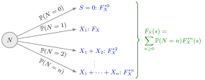
$Tree from the claim count N to the cases N = 0, 1, 2 up to n with weights P(N = n), each giving a sum of n severities with law F_X^{*n}, all combined by a brace into F_S.$

The figure reads the formula for $F_S$ as a two-stage experiment. The count is drawn first, with probability $\mathbb{P}(N=n)$ for each branch; given $N=n$ $n$ , the loss is a sum of $n$ independent severities, whose law is the $n$ -fold convolution $F_X^{*n}$ (and $S=0$ when $n=0$ $0$ ). Averaging the branch laws with the branch probabilities gives $F_S$ . In the Bernoulli Example only the branches $n=0$ and $n=1$ remain, with weights $1-q$ and $q$ , which is why the result is a simple mixture.

Pick a claim-count law and move $\mathbb E[N]$ : the count's variance enters $\operatorname{Var}(S)=\mathbb E[N]\sigma^2+\operatorname{Var}(N)\mu^2$ $Var (N) μ^{2}$ . With a Bernoulli count $S$ is 0 with probability $1-q$ and otherwise one severity.

The collective risk model supplies the random-sum assumptions. Given $N=n$ $n$ , convolution of independent random variables gives $F_X^{*n}$ , and the probability generating function averages transform powers over the count. Adam’s law: total expectation applied to $\mathbb{E}[S\mid N]=N\mu$ gives the mean. The conditioning trick for variance combines $\operatorname{Var}(S\mid N)=N\sigma^2$ with variation in $N\mu$ to give the two variance terms.

Key Results¶

$\mathbb{E}[S]=\mathbb{E}[N]\mu$ $E [N] μ$ .
$\operatorname{Var}(S)=\mathbb{E}[N]\sigma^2+\operatorname{Var}(N)\mu^2$ $Var (N) μ^{2}$ , with finite second moments.
With moment generating function (MGF) $M$ and PGF $G$ , $M_S(t)=G_N(M_X(t))$ where the expression is finite; for integer severities $G_S(z)=G_N(G_X(z))$ $G_{N} (G_{X} (z))$ .
$\displaystyle F_S(s)=\sum_{n\ge0}\mathbb{P}(N=n)F_X^{*n}(s)$ $n) F_{X}^{* n} (s)$ , with $F_X^{*0}$ the cumulative distribution function of the constant zero.

Examples¶

If $N$ is Bernoulli with probability $q$ , then $S$ is zero with probability $1-q$ and otherwise has the severity law. Thus a compound Bernoulli model is also a simple mixture.

Prerequisites¶

Sources¶

Risk Insurance · Lecture 4

Aliases: random sum distribution, compound frequency-severity distribution, compound distribution, random sum, compound sum, stopped-sum distribution Keywords: E[S] = E[N] μ, Var(S) = E[N] σ^2 + Var(N) μ^2, M_S(t) = G_N(M_X(t)), n-fold convolution, compound Bernoulli Symbols: mu, sigma, sum

Last updated: 17 October 2026 21:53