Singular Value Decomposition¶

Theorem¶

Let $A$ be a real $m\times n$ matrix of rank $r$ and $p=\min(m,n)$ $min (m, n)$ . Then

A=U\Sigma V^{\top},

where $U$ ( $m \times$ $m\times m$ $m$ ) and $V$ ( $n \times$ $n\times n$ $n$ ) are orthogonal, $U^{\top}U=I_m$ $I_{m}$ , $V^{\top}V=I_n$ $I_{n}$ , and $\Sigma$ is $m\times n$ with diagonal entries $\sigma_1\ge\cdots\ge\sigma_r>0=\sigma_{r+1}=\cdots=\sigma_p$ and zeros off the diagonal. The $\sigma_i$ are the singular values of $A$ ; the columns $\boldsymbol{u}_i$ of $U$ and $\boldsymbol{v}_i$ of $V$ are the left and right singular vectors. The factorization is the singular value decomposition (SVD) of $A$ .

Interpretation¶

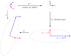
Every linear map $\boldsymbol{x}\mapsto A\boldsymbol{x}$ is a rotation or reflection ( $V^{\top}$ ), then a scaling of the coordinate axes by $\sigma_i$ , possibly with a change of dimension ( $\Sigma$ ), then another rotation or reflection ( $U$ ). The unit sphere is mapped onto an ellipsoid, possibly flattened, with semi-axes $\sigma_i\boldsymbol{u}_i$ .

The unit circle with v_1 and v_2 is sent by V^T to e_1 and e_2, stretched by Σ into an ellipse with semi-axes 3√5 and √5, and moved by U onto the image ellipse of A.

The figure follows the $2\times2$ example below, $A=\begin{pmatrix}3&0\\4&5\end{pmatrix}$ $(3405)$ , with all four panels drawn to the same scale. $V^{\top}$ sends the right singular vectors $\boldsymbol{v}_1,\boldsymbol{v}_2$ to the standard basis vectors $\boldsymbol{e}_1,\boldsymbol{e}_2$ ; $\Sigma$ stretches them to lengths $\sigma_1=3\sqrt{5}$ and $\sigma_2=\sqrt{5}$ $5$ ; $U$ moves the axes onto $\boldsymbol{u}_1,\boldsymbol{u}_2$ . The result is the image of the unit circle under $A$ , with semi-axes $\sigma_1\boldsymbol{u}_1=A\boldsymbol{v}_1$ and $\sigma_2\boldsymbol{u}_2=A\boldsymbol{v}_2$ $A v_{2}$ . In this example $U$ and $V$ both have determinant $-1$ , so both outer steps are reflections.

Turn the unit vector $\boldsymbol{x}$ with $\varphi$ and step through $V^T\boldsymbol{x}$ , $\Sigma V^T\boldsymbol{x}$ and $U\Sigma V^T\boldsymbol{x}$ : a rotation, a stretch by $\sigma_1=3\sqrt5$ and $\sigma_2=\sqrt5$ along the axes, and a second rotation turn the unit circle into the ellipse.

The proof is constructive. $A^{\top}A$ is symmetric and positive semidefinite, so its orthogonal diagonalization supplies orthonormal eigenvectors $\boldsymbol{v}_i$ with eigenvalues $\sigma_i^2$ . Then $\boldsymbol{u}_i=A\boldsymbol{v}_i/\sigma_i$ for $i\le r$ are orthonormal, and the Gram-Schmidt algorithm completes them to an orthonormal basis of $\mathbb{R}^m$ .

Unlike diagonalization $P^{-1}AP$ , the SVD exists for every matrix, square or not, and uses two different orthonormal bases. It coincides with the spectral decomposition only for symmetric positive semidefinite matrices; for a symmetric matrix in general $\sigma_i=|\lambda_i|$ $∣ λ_{i} ∣$ .

Key Results¶

$A^{\top}A=V\Sigma^{\top}\Sigma V^{\top}$ and $AA^{\top}=U\Sigma\Sigma^{\top}U^{\top}$ $U Σ Σ^{⊤} U^{⊤}$ ; both have nonzero eigenvalues $\sigma_1^2,\ldots,\sigma_r^2$ , and all their other eigenvalues are $0$ .
$A\boldsymbol{v}_i=\sigma_i\boldsymbol{u}_i$ and $A^{\top}\boldsymbol{u}_i=\sigma_i\boldsymbol{v}_i$ for $i\le p$ $p$ .
Rank-one expansion and reduced SVD: $\displaystyle A=\sum_{i=1}^r\sigma_i\boldsymbol{u}_i\boldsymbol{v}_i^{\top}=U_r\Sigma_rV_r^{\top}$ $U_{r} Σ_{r} V_{r}^{⊤}$ , using only the first $r$ columns.
Orthonormal bases of the four subspaces (Fundamental Theorem of Linear Algebra): $\boldsymbol{u}_1,\ldots,\boldsymbol{u}_r$ for $\operatorname{Col}(A)$ , $\boldsymbol{u}_{r+1},\ldots,\boldsymbol{u}_m$ for $\operatorname{Null}(A^{\top})$ , $\boldsymbol{v}_1,\ldots,\boldsymbol{v}_r$ for $\operatorname{Row}(A)$ , $\boldsymbol{v}_{r+1},\ldots,\boldsymbol{v}_n$ for $\operatorname{Null}(A)$ .
The singular values are unique; $U$ and $V$ are not (signs can be flipped in pairs $\boldsymbol{u}_i,\boldsymbol{v}_i$ , and repeated or zero singular values allow more freedom).
The Moore-Penrose inverse is $A^+=V\Sigma^+U^{\top}$ $V Σ^{+} U^{⊤}$ .

Beyond the course

Many textbooks add the Eckart-Young theorem: keeping only the first $k<r$ terms of the rank-one expansion gives the best approximation of $A$ by a matrix of rank at most $k$ . Math V does not cover it.

Examples¶

A $2\times2$ matrix. For $A=\begin{pmatrix}3&0\\4&5\end{pmatrix}$ $(3405)$ , $A^{\top}A=\begin{pmatrix}25&20\\20&25\end{pmatrix}$ with eigenvalues $45$ and $5$ and eigenvectors $\boldsymbol{v}_1=\tfrac{1}{\sqrt{2}}(1,1)^{\top}$ $\frac{1}{2} (1, 1)^{⊤}$ , $\boldsymbol{v}_2=\tfrac{1}{\sqrt{2}}(1,-1)^{\top}$ $\frac{1}{2} (1, - 1)^{⊤}$ . So $\sigma_1=3\sqrt{5}$ $35$ , $\sigma_2=\sqrt{5}$ $5$ , and

\boldsymbol{u}_1=\frac{A\boldsymbol{v}_1}{\sigma_1}=\frac{(3,9)^{\top}}{\sqrt{2}\cdot3\sqrt{5}} =\tfrac{1}{\sqrt{10}}(1,3)^{\top},\qquad \boldsymbol{u}_2=\frac{A\boldsymbol{v}_2}{\sigma_2}=\tfrac{1}{\sqrt{10}}(3,-1)^{\top}.

Check: $\boldsymbol{u}_1^{\top}\boldsymbol{u}_2=0$ and $\sigma_1\sigma_2=15=|\det A|$ $∣ det A ∣$ .

A rectangular rank-one matrix. $A=\begin{pmatrix}1&1\\1&1\\0&0\end{pmatrix}$ has $A^{\top}A=\begin{pmatrix}2&2\\2&2\end{pmatrix}$ $(2222)$ , eigenvalues $4,0$ . Hence $\sigma_1=2$ $2$ , $\sigma_2=0$ $0$ , $\boldsymbol{v}_1=\tfrac{1}{\sqrt{2}}(1,1)^{\top}$ $\frac{1}{2} (1, 1)^{⊤}$ , $\boldsymbol{u}_1=\tfrac{1}{\sqrt{2}}(1,1,0)^{\top}$ $\frac{1}{2} (1, 1, 0)^{⊤}$ , and $A=2\boldsymbol{u}_1\boldsymbol{v}_1^{\top}$ $2 u_{1} v_{1}^{⊤}$ . Completing with $\boldsymbol{v}_2=\tfrac{1}{\sqrt{2}}(1,-1)^{\top}$ and $\boldsymbol{u}_2=\tfrac{1}{\sqrt{2}}(1,-1,0)^{\top}$ $\frac{1}{2} (1, - 1, 0)^{⊤}$ , $\boldsymbol{u}_3=(0,0,1)^{\top}$ gives the full SVD with $\Sigma=\begin{pmatrix}2&0\\0&0\\0&0\end{pmatrix}$ $200000$ .

Prerequisites¶

Sources¶

Math V: Advanced Linear Algebra · Week 7

Aliases: SVD, singular value decomposition theorem Keywords: A = U Σ V^T, left singular vectors, right singular vectors, reduced SVD, thin SVD, rank-one expansion, Eckart-Young Symbols: lambda, phi, real numbers, sigma, square root, sum

Last updated: 22 October 2026 19:04