First-Order Linear Difference Equation¶

Definition¶

A first-order linear difference equation with constant coefficient is

x_{t+1}=a\,x_t+g_t,\qquad t=0,1,2,\ldots,

where $a\ne0$ is a real constant and $(g_t)_{t\ge0}$ is a given forcing sequence. It is homogeneous if $g_t=0$ for all $t$ . For every initial value $x_0$ the unique solution is

x_t=a^t x_0+\sum_{s=0}^{t-1}a^{\,t-1-s}\,g_s.

Interpretation¶

The next state is the current state scaled by $a$ plus an external input. The solution formula is obtained by substituting the equation into itself: the initial value is multiplied by $a$ once per period, and the input $g_s$ received at time $s$ has been multiplied by $a$ for the remaining $t-1-s$ periods.

Two paths from x_0 = 10 to the dashed equilibrium x* = 6: for a = 0.5 the values fall monotonically, for a = -0.5 they jump above and below 6 while closing in.

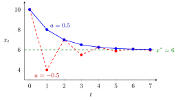
The figure shows two solutions with constant input, both starting at $x_0=10$ and both with the equilibrium (constant solution) $x^*=6$ $6$ , dashed. The blue path is the convergent example $x_{t+1}=0.5x_t+3$ $3$ , that is $x_t=6+4(0.5)^t$ $4 (0.5)^{t}$ , which falls monotonically ( $10,8,7,6.5,\ldots$ ). The red path is $x_{t+1}=-0.5x_t+9$ $9$ , which has the same equilibrium $9/1.5=6$ $6$ ; here $x_t=6+4(-0.5)^t$ alternates ( $10,4,7,5.5,\ldots$ ). Both transients shrink by the factor $\lvert a\rvert=0.5$ per period.

Move $a$ , $b$ and $x_0$ : for $|a|<1$ the path settles on the dashed equilibrium $x^*=b/(1-a)$ $a)$ , monotonically when $a>0$ and alternating around $x^*$ when $a<0$ $0$ . At $a=1$ with $b\ne0$ there is no equilibrium and the path grows linearly.

With a constant input $g_t=b$ and $a\ne1$ $1$ , the constant $x^*=b/(1-a)$ is the unique equilibrium, and the deviation $x_t-x^*$ satisfies the homogeneous equation. Hence $x_t=x^*+a^t(x_0-x^*)$ $x^{*})$ : an equilibrium plus a transient. The size of $\lvert a\rvert$ decides whether the transient dies out (see stability of a scalar difference equation), and the sign of $a$ decides whether the path is monotone ( $a >$ $a>0$ $0$ ) or alternates around $x^*$ ( $a <$ $a<0$ $0$ ).

The case $a=1$ is different: there is no equilibrium when $b\ne0$ $0$ , and $x_t=x_0+bt$ grows linearly. Forgetting this case, and dividing by $1-a=0$ $0$ , is a common error.

Key Results¶

Homogeneous case: $x_t=a^t x_0$ $a^{t} x_{0}$ , a geometric sequence.
Constant input $b$ , $a\ne1$ $1$ : $x_t=\dfrac{b}{1-a}+a^t\Big(x_0-\dfrac{b}{1-a}\Big)$ $\frac{b}{1 - a})$ ; by the geometric series formula, $\displaystyle \sum_{s=0}^{t-1}a^{t-1-s}b=b\,\dfrac{1-a^t}{1-a}$ $b \frac{1 - a ^{t}}{1 - a}$ .
Constant input $b$ , $a=1$ $1$ : $x_t=x_0+bt$ $b t$ .
If $\lvert a\rvert<1$ and $g_t=b$ $b$ , then $x_t\to b/(1-a)$ for every $x_0$ ; if $\lvert a\rvert>1$ $1$ , the path diverges unless $x_0=x^*$ $x^{*}$ .
$a=-1$ gives a two-cycle $x_t=x^*+(-1)^t(x_0-x^*)$ around $x^*=b/2$ (a constant path if $x_0=x^*$ $x^{*}$ ).

Examples¶

Convergent case. $x_{t+1}=0.5x_t+3$ $3$ , $x_0=10$ $10$ . The equilibrium is $x^*=3/(1-0.5)=6$ $6$ , so $x_t=6+4(0.5)^t$ $4 (0.5)^{t}$ . Check: $x_1=0.5\cdot10+3=8=6+4\cdot0.5$ $0.5$ , and $x_t\to6$ $6$ .

Savings account. A balance earning $5\%$ per period with a deposit of $100$ at the end of each period satisfies $B_{t+1}=1.05B_t+100$ $100$ , $B_0=0$ $0$ . Here $x^*=100/(1-1.05)=-2000$ $- 2000$ , so $B_t=2000(1.05^t-1)$ $1)$ . Check: $B_1=100$ and $B_2=2000\cdot0.1025=205=1.05\cdot100+100$ $100$ . The equilibrium is negative and unstable: it only describes the path, not a long-run level.

Time-varying input. $x_{t+1}=2x_t+t$ $t$ , $x_0=0$ $0$ : the formula gives $x_3=2^2\cdot0+2^1\cdot1+2^0\cdot2=4$ $4$ , matching the recursion $x_1=0$ $0$ , $x_2=1$ $1$ , $x_3=2\cdot1+2=4$ $4$ .

Prerequisites¶

Sources¶

Math V: Advanced Linear Algebra · Week 2

Aliases: First Order Linear Difference Equation, first-order linear recurrence, linear difference equation of order one, linear first-order difference equation Keywords: x_{t+1} = a x_t + g_t, x_t = a^t x_0, equilibrium b/(1-a), steady state, forcing term Symbols: sum

Last updated: 17 October 2026 21:53