Integrating Factor¶

Method¶

Consider the linear first-order differential equation

x'(t)+p(t)\,x(t)=q(t),\qquad t\in I,

with $p,q$ continuous on an interval $I$ and $x'(t)=\dfrac{\mathrm{d}x}{\mathrm{d}t}(t)$ $\frac{d x}{d t} (t)$ .

Choose an antiderivative $P$ of $p$ and set $\mu(t)=\mathrm{e}^{P(t)}$ $e^{P (t)}$ , the integrating factor.
Multiply the equation by $\mu(t)$ . Since $\mu'(t)=p(t)\mu(t)$ $p (t) μ (t)$ , the left-hand side becomes an exact derivative: $\mu x'+\mu p x=(\mu x)'$ $(μx)^{'}$ .
Integrate $(\mu x)'=\mu q$ $μ q$ : $\ \mu(t)x(t)=\int\mu(t)q(t)\,\mathrm{d}t+C$ $C$ .
Divide by $\mu(t)>0$ $0$ : $\ x(t)=\mathrm{e}^{-P(t)}\Big(\int \mathrm{e}^{P(t)}q(t)\,\mathrm{d}t+C\Big)$ $C)$ , and fix $C$ from an initial condition.

With $x(t_0)=x_0$ and $P(t_0)=0$ this gives the closed form

x(t)=\mathrm{e}^{-P(t)}x_0 +\int_{t_0}^{t}\mathrm{e}^{-(P(t)-P(s))}\,q(s)\,\mathrm{d}s.

Interpretation¶

The left-hand side $x'+px$ is not a derivative of anything simple; multiplying by $\mu$ turns it into the derivative of the product $\mu x$ . Step 2 uses the product rule from differentiation rules and the chain rule for $\frac{\mathrm{d}}{\mathrm{d}t}\mathrm{e}^{P(t)}=P'(t)\mathrm{e}^{P(t)}$ $P^{'} (t) e^{P (t)}$ .

The two terms of the closed form have a meaning: $\mathrm{e}^{-P(t)}x_0$ solves the homogeneous equation $x'+px=0$ $0$ , and the integral is a particular solution that starts at $0$ , so the solution is homogeneous part plus particular part, as in the general solution of a linear ODE. For constant $p=-a$ the formula reads $x(t)=\mathrm{e}^{a(t-t_0)}x_0+\int_{t_0}^t \mathrm{e}^{a(t-s)}q(s)\,\mathrm{d}s$ $\int_{t_{0}}^{t} e^{a (t - s)} q (s) d s$ , the scalar form of the variation-of-constants formula that returns in Week 4 with the matrix exponential.

Common slips: forgetting to write the equation with coefficient $1$ in front of $x'$ before reading off $p$ ; using $\mathrm{e}^{-P}$ instead of $\mathrm{e}^{P}$ ; adding the constant $C$ after dividing by $\mu$ instead of before.

Key Results¶

$\mu(t)=\mathrm{e}^{P(t)}$ is never zero, so multiplying by it neither loses nor creates solutions.
Any antiderivative of $p$ can be used: replacing $P$ by $P+k$ multiplies $\mu$ by $\mathrm{e}^{k}$ , which cancels.
If $p,q$ are continuous on $I$ , the method yields the unique solution of each initial value problem on all of $I$ .
For constant $p\neq0$ and constant $q$ the solution tends to $q/p$ when $p>0$ $0$ ; this limit is the equilibrium.

Examples¶

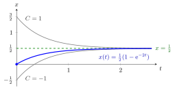
Constant coefficients. $x'+2x=1$ $1$ , $x(0)=0$ $0$ . Take $\mu=\mathrm{e}^{2t}$ $e^{2 t}$ : $(\mathrm{e}^{2t}x)'=\mathrm{e}^{2t}$ $e^{2 t}$ , so $\mathrm{e}^{2t}x=\tfrac{1}{2}\mathrm{e}^{2t}+C$ and $x=\tfrac{1}{2}+C\mathrm{e}^{-2t}$ $C e^{- 2 t}$ . From $x(0)=0$ $0$ , $C=-\tfrac{1}{2}$ $- \frac{1}{2}$ : $x(t)=\tfrac{1}{2}(1-\mathrm{e}^{-2t})$ $e^{- 2 t})$ .

Solution curves x = 1/2 + Ce^(-2t) of x' + 2x = 1 for C = 1, -1/2 and -1, all approaching the dashed line x = 1/2, with the solution through x(0) = 0 highlighted.

The figure plots the general solution $x=\tfrac{1}{2}+C\mathrm{e}^{-2t}$ for $C=1$ $1$ , $C=-\tfrac{1}{2}$ and $C=-1$ $- 1$ . The constant $C$ only shifts the decaying homogeneous part $C\mathrm{e}^{-2t}$ , so every curve approaches the equilibrium $x=\tfrac{1}{2}=q/p$ $q / p$ ; the initial condition $x(0)=0$ picks out the highlighted curve with $C=-\tfrac{1}{2}$ $- \frac{1}{2}$ .

Move $x(0)$ to change the constant $C$ in $x=q/p+C\mathrm{e}^{-pt}$ $C e^{- pt}$ : for $p>0$ every solution approaches the dashed level $q/p$ . Then change $p$ and $q$ .

Variable coefficient. $x'+\frac{1}{t} x=t$ on $t>0$ $0$ . Here $P(t)=\ln t$ and $\mu=t$ $t$ : $(tx)'=t^2$ $t^{2}$ , so $tx=\tfrac{t^3}{3}+C$ and $x(t)=\tfrac{t^2}{3}+\tfrac{C}{t}$ $\frac{C}{t}$ . Check: $x'+\frac{x}{t}=\tfrac{2t}{3}-\tfrac{C}{t^2}+\tfrac{t}{3}+\tfrac{C}{t^2}=t$ $t$ .

With integration by parts. $x'-x=t$ $t$ . Here $\mu=\mathrm{e}^{-t}$ and $(\mathrm{e}^{-t}x)'=t\mathrm{e}^{-t}$ $t e^{- t}$ . Integration by parts gives $\int t\mathrm{e}^{-t}\,\mathrm{d}t=-t\mathrm{e}^{-t}-\mathrm{e}^{-t}+C$ $C$ , so $x(t)=-t-1+C\mathrm{e}^{t}$ $C e^{t}$ . Check: $x'=-1+C\mathrm{e}^t$ and $x+t=-1+C\mathrm{e}^t$ $C e^{t}$ .

Prerequisites¶

Sources¶

Math V: Advanced Linear Algebra · Week 3

Aliases: integrating factor method, method of integrating factors Keywords: mu(t)=e^{P(t)}, x'+p(t)x=q(t), linear first-order equation, variation of constants, product rule Symbols: element of, integral, mu

Last updated: 22 October 2026 19:04