Least Squares¶

Method¶

Let $A$ be a real $m\times n$ matrix and $\boldsymbol{b}\in\mathbb{R}^m$${\mathbb{R}}^m$. A least-squares solution of $A\boldsymbol{x}=\boldsymbol{b}$ is a vector $\hat{\boldsymbol{x}}\in\mathbb{R}^n$ such that, for all $\boldsymbol{x}\in\mathbb{R}^n$${\mathbb{R}}^n$,

where $\|\cdot\|$ is the Euclidean norm. To find it, solve the normal equations

The vector $\boldsymbol{b}-A\hat{\boldsymbol{x}}$ is the residual.

Interpretation¶

When $\boldsymbol{b}$ is not in the column space $\operatorname{Col}(A)$ (the range of $A$), the system has no solution, typically because there are more equations than unknowns. Least squares replaces $\boldsymbol{b}$ by the closest attainable vector, the orthogonal projection $\boldsymbol{p}$ of $\boldsymbol{b}$ onto $\operatorname{Col}(A)$, and solves $A\hat{\boldsymbol{x}}=\boldsymbol{p}$$\mathbf{p}$.

The normal equations say that the residual is orthogonal to every column, since the rows of the transpose are the columns of $A$: $A^{\top}(\boldsymbol{b}-A\hat{\boldsymbol{x}})=\boldsymbol{0}$$0$, that is, the residual lies in $\operatorname{Null}(A^{\top})=\operatorname{Col}(A)^\perp$ given by the Fundamental Theorem of Linear Algebra. The same equations follow from setting the gradient of $\|\boldsymbol{b}-A\boldsymbol{x}\|^2$$A\mathbf{x}{\Vert }^2$, namely $2A^{\top}A\boldsymbol{x}-2A^{\top}\boldsymbol{b}$$2A^{\top }\mathbf{b}$, to zero.

Misunderstandings to avoid: the fitted vector $A\hat{\boldsymbol{x}}$ is always unique, but $\hat{\boldsymbol{x}}$ need not be; and the formula $(A^{\top}A)^{-1}A^{\top}\boldsymbol{b}$ is valid only when the columns of $A$ are linearly independent.

Key Results¶

• The normal equations are always consistent, and their solution set equals the set of least-squares solutions.
• Since $\operatorname{Null}(A^{\top}A)=\operatorname{Null}(A)$$\mathrm{Null}(A)$, the least-squares solutions form the affine subspace $\{\hat{\boldsymbol{x}}\}+\operatorname{Null}(A)$$\mathrm{Null}(A)$.
• The solution is unique if and only if $A$ has full column rank $n$; then $\hat{\boldsymbol{x}}=(A^{\top}A)^{-1}A^{\top}\boldsymbol{b}$ and $\boldsymbol{p}=H\boldsymbol{b}$ with the symmetric idempotent matrix $H=A(A^{\top}A)^{-1}A^{\top}$$A(A^{\top }A{)}^{-1}{A}^{\top }$.
• In general, $\hat{\boldsymbol{x}}^+=A^+\boldsymbol{b}$$A^{+}\mathbf{b}$, with $A^+$ the Moore-Penrose inverse, is the unique least-squares solution of minimum norm; it is the one lying in the row space $\operatorname{Row}(A)$.

Examples¶

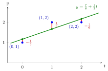
Fitting a line. Fit $y=c_0+c_1t$ to the points $(0,1),(1,2),(2,2)$. Then

Solving $3c_0+3c_1=5$$5$, $3c_0+5c_1=6$ gives $c_1=\tfrac{1}{2}$$\frac{1}{2}$, $c_0=\tfrac{7}{6}$$\frac{7}{6}$. The fitted values are $(\tfrac{7}{6},\tfrac{5}{3},\tfrac{13}{6})^{\top}$, the residual is $(-\tfrac{1}{6},\tfrac{1}{3},-\tfrac{1}{6})^{\top}$, whose entries sum to $0$ and are orthogonal to $(0,1,2)^{\top}$, and the minimal sum of squares is $\tfrac{1}{6}$.

In the figure, the residuals are the vertical gaps between the data and the fitted line, $-\tfrac{1}{6}$, $\tfrac{1}{3}$ and $-\tfrac{1}{6}$. Their squares add up to $\tfrac{1}{6}$, and no other line does better. Seen in $\mathbb{R}^3$, the fitted values $(\tfrac{7}{6},\tfrac{5}{3},\tfrac{13}{6})^{\top}$ are the orthogonal projection of $\boldsymbol{b}$ onto $\operatorname{Col}(A)$, and the residual vector is orthogonal to both columns of $A$.

Rank-deficient case. For $A=\begin{pmatrix}1&1\\1&1\end{pmatrix}$$\left(\begin{array}{cc}1& 1\\ 1& 1\end{array}\right)$, $\boldsymbol{b}=(1,3)^{\top}$$(1,3{)}^{\top }$: the normal equations reduce to $x_1+x_2=2$$2$, so every $(2-t,t)^{\top}$ is a least-squares solution, with fitted vector $(2,2)^{\top}$, the projection of $\boldsymbol{b}$ onto $\operatorname{span}\{(1,1)^{\top}\}$. The minimum-norm solution is $(1,1)^{\top}=A^+\boldsymbol{b}$$A^{+}\mathbf{b}$, using $A^+=\tfrac{1}{4}A$$\frac{1}{4}A$.

Prerequisites¶

• Euclidean Norm
• Range of a Linear Map
• Transpose
• Orthogonal Projection
• Fundamental Theorem of Linear Algebra

Related Concepts¶

• Moore-Penrose Inverse
• Singular Value Decomposition
• Gram-Schmidt Algorithm
• Idempotent Matrix

Sources¶

• Math V: Advanced Linear Algebra · Week 7

Aliases: method of least squares, linear least squares, least-squares solution, least-squares method, least-squares problem, least-squares approximation Keywords: normal equations, A^T A x = A^T b, (A^T A)^{-1} A^T b, residual, minimum-norm least-squares solution, A^+ b, line fitting Symbols: element of, real numbers

Last updated: 22 October 2026 19:04