Second-Order Differential Equation¶

Definition¶

A second-order differential equation is a differential equation in which the second derivative $x''(t)$ is the highest higher-order derivative of the unknown $x(t)$ that occurs; explicitly, $x''(t)=f\big(t,x(t),x'(t)\big)$ $f (t, x (t), x^{'} (t))$ , where $x'(t)=\dfrac{\mathrm{d}x}{\mathrm{d}t}(t)$ $\frac{d x}{d t} (t)$ .

It is linear if it can be written as

x''(t)+a_1(t)\,x'(t)+a_0(t)\,x(t)=g(t),

with constant coefficients if $a_1,a_0$ are constants, and homogeneous if $g\equiv0$ $0$ . An initial value problem prescribes two initial conditions, $x(t_0)=x_0$ and $x'(t_0)=v_0$ $v_{0}$ .

Interpretation¶

The state of a second-order system at time $t$ is the pair $\big(x(t),x'(t)\big)$ , position and velocity in mechanics. Knowing only $x(t_0)$ is not enough: a pendulum released at the same position with different velocities moves differently. This is why two constants appear in the general solution, compared with one for a first-order differential equation.

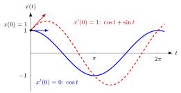
Two solutions of x'' + x = 0 start at x(0) = 1: the cosine has initial velocity 0, and the dashed curve cos t + sin t has initial velocity 1.

Both curves solve $x''+x=0$ and start at the same position $x(0)=1$ $1$ . With $x'(0)=0$ the solution is $\cos t$ , as in the first example below; with $x'(0)=1$ the conditions give $c_1=1$ $1$ , $c_2=1$ $1$ , so $x(t)=\cos t+\sin t$ $sin t$ . The arrows show the two initial slopes: the same position with a different velocity gives a different solution, so both $x(t_0)$ and $x'(t_0)$ must be prescribed.

Change $x'(0)$ to see that the position $x(0)$ alone does not fix the solution. Then move $a_1$ and $a_0$ : the roots of $r^2+a_1r+a_0=0$ decide whether $x(t)$ oscillates, decays or grows.

Setting $y_1=x$ and $y_2=x'$ rewrites the constant-coefficient equation $x''+a_1x'+a_0x=g$ as a first-order system

\begin{pmatrix}y_1\\y_2\end{pmatrix}'=\begin{pmatrix}0&1\\-a_0&-a_1\end{pmatrix}\begin{pmatrix}y_1\\y_2\end{pmatrix}+\begin{pmatrix}0\\g\end{pmatrix}.

The eigenvalues $\lambda$ of this companion matrix satisfy $\lambda^2+a_1\lambda+a_0=0$ $0$ , which is the characteristic equation of the scalar equation. Here the scalar and the matrix viewpoints meet.

A frequent slip is to treat the equation as linear when $x$ or $x'$ enters nonlinearly, as in $x''+\sin x=0$ (the exact pendulum) or $x''+x\,x'=0$ $0$ .

Key Results¶

If $a_1,a_0,g$ are continuous on an interval $I$ , each initial value problem with $x(t_0)=x_0$ $x_{0}$ , $x'(t_0)=v_0$ has exactly one solution on $I$ .
The solutions of the homogeneous linear equation form a two-dimensional vector space.
Every solution of the inhomogeneous equation is $x=x_p+c_1x_1+c_2x_2$ $c_{2} x_{2}$ , with $x_p$ a particular solution and $x_1,x_2$ independent homogeneous solutions.
For constant coefficients, the homogeneous solutions come from the roots of $r^2+a_1r+a_0=0$ $0$ .

Examples¶

Undamped oscillation. $x''+x=0$ with $x(0)=1$ $1$ , $x'(0)=0$ $0$ . The functions $\cos t$ and $\sin t$ solve it, so $x=c_1\cos t+c_2\sin t$ $c_{2} sin t$ ; the conditions give $c_1=1$ $1$ , $c_2=0$ $0$ , hence $x(t)=\cos t$ $cos t$ .

Distinct real roots. $x''+3x'+2x=0$ with $x(0)=0$ $0$ , $x'(0)=1$ $1$ . Roots of $r^2+3r+2=(r+1)(r+2)$ are $-1,-2$ , so $x=c_1\mathrm{e}^{-t}+c_2\mathrm{e}^{-2t}$ $c_{2} e^{- 2 t}$ . Then $c_1+c_2=0$ and $-c_1-2c_2=1$ $1$ , giving $c_2=-1$ $- 1$ , $c_1=1$ $1$ : $x(t)=\mathrm{e}^{-t}-\mathrm{e}^{-2t}$ $e^{- 2 t}$ . Check: $x'(0)=-1+2=1$ $1$ .

Repeated root. $x''+2x'+x=0$ has $r^2+2r+1=(r+1)^2$ $1)^{2}$ , a double root $-1$ , and the solution basis $\mathrm{e}^{-t}$ , $t\mathrm{e}^{-t}$ .

Pure forcing. $x''=-c$ with a constant $c$ (free fall under constant gravity) with $x(0)=x_0$ $x_{0}$ , $x'(0)=v_0$ integrates twice to $x(t)=x_0+v_0t-\tfrac{1}{2}ct^2$ $\frac{1}{2} c t^{2}$ .

Prerequisites¶

Sources¶

Math V: Advanced Linear Algebra · Week 4

Aliases: Second Order Differential Equation, second-order ODE, second order ODE Keywords: x''(t)+a_1 x'(t)+a_0 x(t)=g(t), two initial conditions, companion matrix, harmonic oscillator, damped oscillation Symbols: lambda

Last updated: 14 October 2026 08:21