Skip to content

Matrix Exponential


Definition

For a square matrix A∈Rn×nA\in\mathbb{R}^{n\times n} (or Cn×n\mathbb{C}^{n\times n}), the matrix exponential is

eA=∑k=0∞Akk!=I+A+A22!+A33!+⋯ ,\mathrm{e}^{A}=\sum_{k=0}^{\infty}\frac{A^k}{k!} =I+A+\frac{A^2}{2!}+\frac{A^3}{3!}+\cdots,

where A0=IA^0=I and powers are matrix products. For a real variable tt, eAt=∑k≥0tkk!Ak\displaystyle \mathrm{e}^{At}=\sum_{k\geq0}\frac{t^k}{k!}A^k. The series converges entrywise for every square matrix.


Interpretation

The definition copies the Taylor series of the scalar exponential function, ea=∑ak/k!\displaystyle \mathrm{e}^{a}=\sum a^k/k!. Its purpose is the same as in the scalar case: ddteAt=AeAt\frac{\mathrm{d}}{\mathrm{d}t}\mathrm{e}^{At}=A\mathrm{e}^{At}, so eAtx0\mathrm{e}^{At}\boldsymbol{x}_0 solves the linear vector ODE x′(t)=Ax(t)\boldsymbol{x}'(t)=A\boldsymbol{x}(t) with x(0)=x0\boldsymbol{x}(0)=\boldsymbol{x}_0.

The series is rarely summed directly. One computes eAt\mathrm{e}^{At} through diagonalization or the Jordan normal form, because (PDP−1)k=PDkP−1(PDP^{-1})^k=PD^kP^{-1}: the exponential respects a similarity transformation.

The main pitfall: eA\mathrm{e}^{A} is not the matrix of entrywise exponentials (eaij)(\mathrm{e}^{a_{ij}}). For a diagonal matrix the rule is "exponentiate the diagonal entries": the off-diagonal zeros stay 00 rather than becoming e0=1\mathrm{e}^0=1. For a non-diagonal matrix the off-diagonal entries of eA\mathrm{e}^{A} have no entrywise formula (see the examples). Also, eA+B=eAeB\mathrm{e}^{A+B}=\mathrm{e}^{A}\mathrm{e}^{B} can fail when AB≠BAAB\neq BA.


Key Results

  • eO=I\mathrm{e}^{O}=I,  ddteAt=AeAt=eAtA\ \frac{\mathrm{d}}{\mathrm{d}t}\mathrm{e}^{At}=A\mathrm{e}^{At}=\mathrm{e}^{At}A, and eA(s+t)=eAseAt\mathrm{e}^{A(s+t)}=\mathrm{e}^{As}\mathrm{e}^{At}.
  • If AB=BAAB=BA, then eA+B=eAeB\mathrm{e}^{A+B}=\mathrm{e}^{A}\mathrm{e}^{B}.
  • eA\mathrm{e}^{A} is always invertible with (eA)−1=e−A(\mathrm{e}^{A})^{-1}=\mathrm{e}^{-A}, and det⁡eA=etr⁡A\det \mathrm{e}^{A}=\mathrm{e}^{\operatorname{tr}A} (determinant, trace).
  • If A=PDP−1A=PDP^{-1} with D=diag⁡(λ1,…,λn)D=\operatorname{diag}(\lambda_1,\dots,\lambda_n), then eAt=Pdiag⁡(eλ1t,…,eλnt)P−1\mathrm{e}^{At}=P\operatorname{diag}(\mathrm{e}^{\lambda_1t},\dots,\mathrm{e}^{\lambda_nt})P^{-1}; the eigenvalues of eAt\mathrm{e}^{At} are eλit\mathrm{e}^{\lambda_it}.
  • If Nm=ON^m=O (nilpotent), the series stops: eNt=∑k<mtkk!Nk\displaystyle \mathrm{e}^{Nt}=\sum_{k<m}\frac{t^k}{k!}N^k. For a Jordan block λI+N\lambda I+N this gives e(λI+N)t=eλteNt\mathrm{e}^{(\lambda I+N)t}=\mathrm{e}^{\lambda t}\mathrm{e}^{Nt}.

Examples

Diagonal and scalar. ediag⁡(2,−1)t=diag⁡(e2t,e−t)\mathrm{e}^{\operatorname{diag}(2,-1)t}=\operatorname{diag}(\mathrm{e}^{2t},\mathrm{e}^{-t}), and eλIt=eλtI\mathrm{e}^{\lambda It}=\mathrm{e}^{\lambda t}I.

Jordan block. A=(2102)=2I+NA=\begin{pmatrix}2&1\\0&2\end{pmatrix}=2I+N with N=(0100)N=\begin{pmatrix}0&1\\0&0\end{pmatrix}, N2=ON^2=O. Since 2I2I and NN commute,

eAt=e2t(I+tN)=e2t(1t01).\mathrm{e}^{At}=\mathrm{e}^{2t}(I+tN)=\mathrm{e}^{2t}\begin{pmatrix}1&t\\0&1\end{pmatrix}.

Check: det⁡eAt=e4t=etr⁡(At)\det \mathrm{e}^{At}=\mathrm{e}^{4t}=\mathrm{e}^{\operatorname{tr}(At)}.

Diagonalizable. A=(1221)=Pdiag⁡(3,−1)P−1A=\begin{pmatrix}1&2\\2&1\end{pmatrix}=P\operatorname{diag}(3,-1)P^{-1} with P=(111−1)P=\begin{pmatrix}1&1\\1&-1\end{pmatrix}, P−1=12(111−1)P^{-1}=\tfrac{1}{2}\begin{pmatrix}1&1\\1&-1\end{pmatrix}. Then

eAt=12(e3t+e−te3t−e−te3t−e−te3t+e−t),\mathrm{e}^{At}=\frac{1}{2}\begin{pmatrix}\mathrm{e}^{3t}+\mathrm{e}^{-t}&\mathrm{e}^{3t}-\mathrm{e}^{-t}\\\mathrm{e}^{3t}-\mathrm{e}^{-t}&\mathrm{e}^{3t}+\mathrm{e}^{-t}\end{pmatrix},

which equals II at t=0t=0.

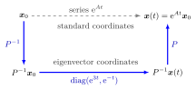
A square diagram: x0 is taken to eigenvector coordinates by P inverse, multiplied by diag(e^3t, e^-t), and returned by P, giving x(t) without summing the series.

The figure shows the route taken in this example. Rather than summing the series for eAt\mathrm{e}^{At} directly (dashed), one passes to eigenvector coordinates with P−1P^{-1}, where the exponential acts as diag⁡(e3t,e−t)\operatorname{diag}(\mathrm{e}^{3t},\mathrm{e}^{-t}), and returns with PP. Both routes give the same x(t)=eAtx0\boldsymbol{x}(t)=\mathrm{e}^{At}\boldsymbol{x}_0 because eAt=Pdiag⁡(e3t,e−t)P−1\mathrm{e}^{At}=P\operatorname{diag}(\mathrm{e}^{3t},\mathrm{e}^{-t})P^{-1}.

Move tt: the point eAtx0e^{At}\boldsymbol{x}_0 runs along the solution curve, its coordinates along the eigenvectors multiplied by e3te^{3t} and e−te^{-t}. At t=0t=0 it is x0\boldsymbol{x}_0 itself, since eO=Ie^{O}=I.

Rotation. For A=(0−110)A=\begin{pmatrix}0&-1\\1&0\end{pmatrix}, A2=−IA^2=-I, and splitting the series into even and odd powers gives eAt=(cos⁡t−sin⁡tsin⁡tcos⁡t)\mathrm{e}^{At}=\begin{pmatrix}\cos t&-\sin t\\\sin t&\cos t\end{pmatrix}, the matrix analogue of Euler's formula.


Prerequisites


Sources

Aliases: exponential of a matrix, e^{At} Keywords: exp(A), e^{At}=Pe^{Dt}P^{-1}, exponential series, nilpotent matrix, det e^A = e^{tr A} Symbols: complex numbers, element of, infinity, lambda, real numbers, sum

Last updated: 22 October 2026 19:04