System of Linear Difference Equations¶

Definition¶

A system of linear difference equations (first order, constant coefficients) is

\boldsymbol{x}_{t+1}=A\boldsymbol{x}_t+\boldsymbol{b}_t,\qquad t=0,1,2,\ldots,

where $\boldsymbol{x}_t\in\mathbb{R}^n$ is the state vector, $A$ is a fixed real $n\times n$ matrix and $(\boldsymbol{b}_t)$ is a given sequence of forcing vectors. It is homogeneous if $\boldsymbol{b}_t=\boldsymbol{0}$ for all $t$ . For every initial vector $\boldsymbol{x}_0$ the unique solution is

\boldsymbol{x}_t=A^t\boldsymbol{x}_0+\sum_{s=0}^{t-1}A^{t-1-s}\boldsymbol{b}_s.

Interpretation¶

Entry $a_{ij}$ says how much variable $j$ today contributes to variable $i$ in the next period. The system is the vector form of the first-order linear difference equation: the number $a$ becomes the matrix $A$ , and $a^t$ becomes the matrix power $A^t$ .

The iterates x_0 = (1,0), x_1 = (0.9,0.1), x_2, … of the population-shares system move along the dashed line x_1 + x_2 = 1 towards x* = (2/3,1/3) on the line through (2,1).

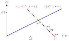
The figure plots the population-shares example below. Writing $\boldsymbol{x}_0=(1,0)^{\top}$ in the eigenvector basis, the component along $(2,1)^{\top}$ ( $λ =$ $\lambda=1$ $1$ ) never changes, while the component along $(1,-1)^{\top}$ ( $λ =$ $\lambda=0.7$ $0.7$ ) is multiplied by $0.7$ each period. So the iterates move along the dashed line through $\boldsymbol{x}_0$ in direction $(1,-1)^{\top}$ , with steps shrinking by the factor $0.7$ , towards $\boldsymbol{x}^*=(2/3,1/3)^{\top}$ on the blue eigenvector line.

Powers of $A$ are hard to read off directly, which is where eigenvalues and eigenvectors come in. If $A\boldsymbol{p}=\lambda\boldsymbol{p}$ $λ p$ , then $A^t\boldsymbol{p}=\lambda^t\boldsymbol{p}$ $λ^{t} p$ : along an eigenvector the system behaves like a scalar equation. When $A$ has $n$ independent eigenvectors, write $\boldsymbol{x}_0$ in that basis and each component evolves separately. This is diagonalization applied to dynamics.

Any scalar linear constant-coefficient higher-order equation can be written as such a system with a companion matrix, so the system covers every linear constant-coefficient difference equation. A common mistake is to compute $A^t$ entrywise. For a diagonal matrix and a positive integer $t$ , raise each diagonal entry to the power $t$ and leave the off-diagonal entries zero. Entrywise powers are not a general rule for other matrices, although special nondiagonal matrices can also satisfy it.

Key Results¶

If $A=PDP^{-1}$ with $D=\operatorname{diag}(\lambda_1,\ldots,\lambda_n)$ $diag (λ_{1}, \dots, λ_{n})$ , then $A^t=PD^tP^{-1}$ and the homogeneous solution is $\displaystyle \boldsymbol{x}_t=\sum_{i=1}^n c_i\lambda_i^t\boldsymbol{p}_i$ with $\boldsymbol{c}=P^{-1}\boldsymbol{x}_0$ $P^{- 1} x_{0}$ .
For a nondiagonalizable $A$ , the Jordan normal form adds terms $t^j\lambda^t$ ( $λ \neq =$ $\lambda\ne0$ $0$ ) for $0\le j<$ the size of the Jordan block.
With constant forcing $\boldsymbol{b}$ , an equilibrium solves $(I-A)\boldsymbol{x}^*=\boldsymbol{b}$ $b$ ; it is unique if and only if $1$ is not an eigenvalue of $A$ . Then $\boldsymbol{x}_t-\boldsymbol{x}^*=A^t(\boldsymbol{x}_0-\boldsymbol{x}^*)$ $x^{*})$ .
Nonreal eigenvalues of the real matrix $A$ come in conjugate pairs and produce oscillating real solutions.
The long-run behaviour is governed by the eigenvalues of largest modulus; see stability.

Examples¶

Diagonalizable system. Let $A=\begin{pmatrix}2&1\\1&2\end{pmatrix}$ $(2112)$ , with eigenvalues $3,1$ and eigenvectors $\boldsymbol{p}_1=(1,1)^{\top}$ $(1, 1)^{⊤}$ , $\boldsymbol{p}_2=(1,-1)^{\top}$ $(1, - 1)^{⊤}$ . For $\boldsymbol{x}_0=(3,1)^{\top}=2\boldsymbol{p}_1+\boldsymbol{p}_2$ $p_{2}$ ,

\boldsymbol{x}_t=2\cdot3^t\begin{pmatrix}1\\1\end{pmatrix}+\begin{pmatrix}1\\-1\end{pmatrix}.

Check: $\boldsymbol{x}_1=A\boldsymbol{x}_0=(7,5)^{\top}=(6+1,\,6-1)^{\top}$ $1)^{⊤}$ .

Population shares. Each period $10\%$ of region 1 moves to region 2 and $20\%$ of region 2 moves to region 1: $A=\begin{pmatrix}0.9&0.2\\0.1&0.8\end{pmatrix}$ $(0.9 0.1 0.2 0.8)$ . The eigenvalues are $1$ (eigenvector $(2,1)^{\top}$ ) and $0.7$ (eigenvector $(1,-1)^{\top}$ ). From $\boldsymbol{x}_0=(1,0)^{\top}=\tfrac{1}{3}(2,1)^{\top}+\tfrac{1}{3}(1,-1)^{\top}$ $\frac{1}{3} (1, - 1)^{⊤}$ ,

\boldsymbol{x}_t=\tfrac{1}{3}\begin{pmatrix}2\\1\end{pmatrix}+\tfrac{1}{3}(0.7)^t\begin{pmatrix}1\\-1\end{pmatrix} \to\begin{pmatrix}2/3\\1/3\end{pmatrix}.

Check: $\boldsymbol{x}_1=(0.9,0.1)^{\top}$ both ways. This is a two-state Markov chain written for column vectors.

Prerequisites¶

Sources¶

Math V: Advanced Linear Algebra · Week 2

Aliases: linear system of difference equations, vector difference equation, linear discrete-time system, discrete-time linear system Keywords: x_{t+1} = A x_t + b_t, x_t = A^t x_0, A^t = P D^t P^{-1}, equilibrium (I - A) x* = b, eigenvector decomposition of the solution Symbols: element of, lambda, real numbers, sum

Last updated: 27 October 2026 11:52