Linear Vector ODE¶

Definition¶

A linear vector ODE (ordinary differential equation) with constant coefficients is a system of differential equations of the form

where $\boldsymbol{x}(t)\in\mathbb{R}^n$ is the state vector, $\boldsymbol{x}'(t)$ is its componentwise derivative $\frac{\mathrm{d}}{\mathrm{d}t}\boldsymbol{x}(t)$, and $A\in\mathbb{R}^{n\times n}$ is a constant matrix. The inhomogeneous form is $\boldsymbol{x}'(t)=A\boldsymbol{x}(t)+\boldsymbol{b}(t)$$\mathbf{b}(t)$. An initial value problem fixes $\boldsymbol{x}(0)=\boldsymbol{x}_0$${\mathbf{x}}_0$.

Interpretation¶

The scalar equation $x'=ax$ has solution $\mathrm{e}^{at}x_0$. The vector equation behaves the same way along each eigenvector: if $A\boldsymbol{v}=\lambda\boldsymbol{v}$ (an eigenvalue and eigenvector pair), then $\boldsymbol{x}(t)=\mathrm{e}^{\lambda t}\boldsymbol{v}$ is a solution, because $\boldsymbol{x}'=\lambda \mathrm{e}^{\lambda t}\boldsymbol{v}=\mathrm{e}^{\lambda t}A\boldsymbol{v}=A\boldsymbol{x}$$A\mathbf{x}$. With an eigenbasis, every solution is a combination of such modes.

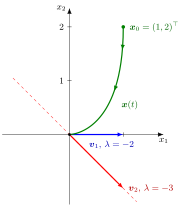
The figure uses the triangular example below, $A=\begin{pmatrix}-2&1\\0&-3\end{pmatrix}$$\left(\begin{array}{cc}-2& 1\\ 0& -3\end{array}\right)$, with eigenvectors $\boldsymbol{v}_1=(1,0)^{\top}$ ($\lambda =$$\lambda=-2$$-2$) and $\boldsymbol{v}_2=(1,-1)^{\top}$ ($\lambda =$$\lambda=-3$$-3$). The solution from $\boldsymbol{x}_0=(1,2)^{\top}$ is $3\mathrm{e}^{-2t}\boldsymbol{v}_1-2\mathrm{e}^{-3t}\boldsymbol{v}_2$$2{\mathrm{e}}^{-3t}{\mathbf{v}}_2$. Both modes decay, so the curve runs into the origin; the $\boldsymbol{v}_2$-mode dies out faster, so the curve arrives along the slower direction $\boldsymbol{v}_1$.

Each eigenvalue $\lambda=\alpha+\mathrm{i}\beta$ contributes the size factor $|\mathrm{e}^{\lambda t}|=\mathrm{e}^{\alpha t}$ and, if $\beta\neq0$$0$, a rotation with angular speed $\beta$. Hence the real parts decide long-run behaviour. This is the continuous-time rule; for difference equations $\boldsymbol{x}_{t+1}=A\boldsymbol{x}_t$ the rule is $|\lambda|<1$ instead (see stability of a system of linear difference equations). Confusing the two is a common error.

The origin $\boldsymbol{0}$ is always an equilibrium of $\boldsymbol{x}'=A\boldsymbol{x}$$A\mathbf{x}$; stability is meant in the sense of stability of an equilibrium.

Key Results¶

• Existence and uniqueness: the initial value problem has the unique solution $\boldsymbol{x}(t)=\mathrm{e}^{At}\boldsymbol{x}_0$${\mathrm{e}}^{At}{\mathbf{x}}_0$, with the matrix exponential.
• If $\boldsymbol{v}_1,\dots,\boldsymbol{v}_n$ is an eigenbasis with eigenvalues $\lambda_1,\dots,\lambda_n$, then $\displaystyle \boldsymbol{x}(t)=\sum_{i=1}^n c_i\mathrm{e}^{\lambda_it}\boldsymbol{v}_i$$\sum _{i=1}^n{c}_i{\mathrm{e}}^{{\lambda }_{i}t}{\mathbf{v}}_i$, with $\boldsymbol{c}$ solving $\displaystyle \sum_ic_i\boldsymbol{v}_i=\boldsymbol{x}_0$${\mathbf{x}}_0$.
• A real matrix with eigenvalue $\alpha+\mathrm{i}\beta$$\mathrm{i}\beta$, $\beta\neq0$$0$, and eigenvector $\boldsymbol{v}$ (its conjugate is then also an eigenvalue, see complex conjugate pair of eigenvalues) gives the two real solutions $\operatorname{Re}\big(\mathrm{e}^{\lambda t}\boldsymbol{v}\big)$ and $\operatorname{Im}\big(\mathrm{e}^{\lambda t}\boldsymbol{v}\big)$, found with Euler's formula.
• If $A$ is not diagonalizable, generalized eigenvectors and the Jordan normal form add terms $t^k\mathrm{e}^{\lambda t}$.
• Stability (stable: all solutions bounded; asymptotically stable: all solutions converge): $\boldsymbol{0}$ is asymptotically stable if and only if every eigenvalue of $A$ has negative real part; it is unstable if some eigenvalue has positive real part. If all real parts are $\leq0$$0$, the origin is stable exactly when each eigenvalue with zero real part has equal algebraic and geometric multiplicity.
• If $A$ is invertible and $\boldsymbol{b}$ is constant, $\boldsymbol{x}^*=-A^{-1}\boldsymbol{b}$ and $\boldsymbol{x}(t)=\boldsymbol{x}^*+\mathrm{e}^{At}(\boldsymbol{x}_0-\boldsymbol{x}^*)$${\mathbf{x}}^{\ast })$.

Examples¶

Triangular matrix. $A=\begin{pmatrix}-2&1\\0&-3\end{pmatrix}$ has eigenvalues $-2,-3$ with eigenvectors $(1,0)^{\top}$ and $(1,-1)^{\top}$. For $\boldsymbol{x}_0=(1,2)^{\top}$$(1,2{)}^{\top }$: $c_1+c_2=1$$1$, $-c_2=2$$2$, so $c_2=-2$$-2$, $c_1=3$ and

Check: $x_1'=-6\mathrm{e}^{-2t}+6\mathrm{e}^{-3t}=-2x_1+x_2$$x_2$. Both eigenvalues are negative, so $\boldsymbol{x}(t)\to\boldsymbol{0}$$0$.

Rotation. $A=\begin{pmatrix}0&-1\\1&0\end{pmatrix}$ has eigenvalues $\pm\mathrm{i}$. The solution $\boldsymbol{x}(t)=\big(x_1(0)\cos t-x_2(0)\sin t,\ x_1(0)\sin t+x_2(0)\cos t\big)^{\top}$ circles the origin with constant length: stable, not asymptotically stable.

Saddle. $A=\begin{pmatrix}1&2\\2&1\end{pmatrix}$ has eigenvalues $3$ and $-1$; the mode $\mathrm{e}^{3t}(1,1)^{\top}$ grows, so the origin is unstable although one eigenvalue is negative.

Prerequisites¶

• System of Differential Equations
• Stability of an Equilibrium
• Eigenvalue and Eigenvector
• Eigenbasis

Related Concepts¶

• Matrix Exponential
• General Solution of a Linear ODE
• Stability of a System of Linear Difference Equations
• Complex Conjugate Pair of Eigenvalues
• Jordan Normal Form

Sources¶

• Math V: Advanced Linear Algebra · Week 4

Aliases: linear system of ODEs, linear vector differential equation, linear system of differential equations Keywords: x'(t)=Ax(t), e^{lambda t} v, eigenvalue solution, asymptotic stability of x' = Ax, negative real part Symbols: alpha, beta, element of, lambda, real numbers, sum

Last updated: 17 October 2026 21:53