Gram-Schmidt Algorithm¶

Method¶

Input: linearly independent vectors $\boldsymbol{a}_1,\ldots,\boldsymbol{a}_k$ in a real inner product space $V$ (in $\mathbb{R}^n$ : the dot product).

Steps: for $j=1,\ldots,k$ $1, \dots, k$ ,

\boldsymbol{v}_j=\boldsymbol{a}_j-\sum_{i=1}^{j-1}\frac{\boldsymbol{a}_j\cdot\boldsymbol{v}_i}{\boldsymbol{v}_i\cdot\boldsymbol{v}_i}\,\boldsymbol{v}_i,\qquad \boldsymbol{q}_j=\frac{\boldsymbol{v}_j}{\|\boldsymbol{v}_j\|}.

Output: orthogonal vectors $\boldsymbol{v}_1,\ldots,\boldsymbol{v}_k$ and orthonormal vectors $\boldsymbol{q}_1,\ldots,\boldsymbol{q}_k$ such that, for every $j$ ,

\operatorname{span}\{\boldsymbol{q}_1,\ldots,\boldsymbol{q}_j\}=\operatorname{span}\{\boldsymbol{a}_1,\ldots,\boldsymbol{a}_j\}.

Interpretation¶

Each step removes from $\boldsymbol{a}_j$ its orthogonal projection onto the span of the earlier vectors; what is left, $\boldsymbol{v}_j$ , is the component of $\boldsymbol{a}_j$ in the orthogonal complement of that span. Dividing by the norm $\|\boldsymbol{v}_j\|=\sqrt{\boldsymbol{v}_j\cdot\boldsymbol{v}_j}$ (the Euclidean norm in $\mathbb{R}^n$ ) then gives a unit vector. Since the $\boldsymbol{q}_i$ are already orthonormal, the update can equally be written $\displaystyle \boldsymbol{v}_j=\boldsymbol{a}_j-\sum_{i<j}(\boldsymbol{a}_j\cdot\boldsymbol{q}_i)\boldsymbol{q}_i$ $q_{i}) q_{i}$ .

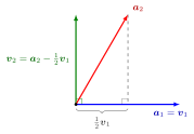
Step two of Gram-Schmidt in the plane of a1 and a2: a2 is dropped perpendicularly onto v1 = a1, the foot is half of v1, and v2 = a2 minus half of v1 is at right angles to v1.

The figure shows the second step of the example below, drawn in the plane spanned by $\boldsymbol{a}_1=(1,1,0)^{\top}$ and $\boldsymbol{a}_2=(1,0,1)^{\top}$ with true lengths. The projection of $\boldsymbol{a}_2$ onto $\boldsymbol{v}_1=\boldsymbol{a}_1$ is $\tfrac{1}{2}\boldsymbol{v}_1$ , since $(\boldsymbol{a}_2\cdot\boldsymbol{v}_1)/(\boldsymbol{v}_1\cdot\boldsymbol{v}_1)=\tfrac{1}{2}$ $\frac{1}{2}$ . Removing it leaves $\boldsymbol{v}_2=\boldsymbol{a}_2-\tfrac{1}{2}\boldsymbol{v}_1=(\tfrac{1}{2},-\tfrac{1}{2},1)^{\top}$ $(\frac{1}{2}, - \frac{1}{2}, 1)^{⊤}$ , the dashed perpendicular moved to the origin, which is orthogonal to $\boldsymbol{v}_1$ .

Linear independence is what guarantees $\boldsymbol{v}_j\neq\boldsymbol{0}$ $0$ , so that the division is allowed. The output depends on the order of the input: reordering the $\boldsymbol{a}_j$ generally gives a different orthonormal basis of the same space.

A frequent slip is to project onto the original $\boldsymbol{a}_i$ instead of the new $\boldsymbol{v}_i$ ; the $\boldsymbol{a}_i$ are not orthogonal, so their projections overlap and the result is wrong.

Key Results¶

$\boldsymbol{v}_j=\boldsymbol{0}$ occurs exactly when $\boldsymbol{a}_j\in\operatorname{span}\{\boldsymbol{a}_1,\ldots,\boldsymbol{a}_{j-1}\}$ $span {a_{1}, \dots, a_{j - 1}}$ ; run on any list, the algorithm detects dependence, and discarding such $\boldsymbol{a}_j$ yields an orthonormal basis of the span of the list.
Every finite-dimensional inner product space has an orthonormal basis, and every orthonormal list extends to one.
In floating-point arithmetic the classical version loses orthogonality; the modified version, which subtracts projections one at a time from the updated vector, is the numerically preferred form.

Beyond the course

Many textbooks collect the Gram-Schmidt output in a factorization $A=QR$ of a matrix with independent columns, with $Q$ having orthonormal columns and $R$ upper triangular. This QR decomposition is not part of Math V.

Examples¶

Three vectors in $\mathbb{R}^3$ . Take $\boldsymbol{a}_1=(1,1,0)^{\top}$ $(1, 1, 0)^{⊤}$ , $\boldsymbol{a}_2=(1,0,1)^{\top}$ $(1, 0, 1)^{⊤}$ , $\boldsymbol{a}_3=(0,1,1)^{\top}$ $(0, 1, 1)^{⊤}$ .

$\boldsymbol{v}_1=(1,1,0)^{\top}$ $(1, 1, 0)^{⊤}$ , $\|\boldsymbol{v}_1\|^2=2$ $2$ .
$\boldsymbol{a}_2\cdot\boldsymbol{v}_1=1$ $1$ , so $\boldsymbol{v}_2=(1,0,1)^{\top}-\tfrac{1}{2}(1,1,0)^{\top}=(\tfrac{1}{2},-\tfrac{1}{2},1)^{\top}$ $(\frac{1}{2}, - \frac{1}{2}, 1)^{⊤}$ , $\|\boldsymbol{v}_2\|^2=\tfrac{3}{2}$ $\frac{3}{2}$ .
$\boldsymbol{a}_3\cdot\boldsymbol{v}_1=1$ and $\boldsymbol{a}_3\cdot\boldsymbol{v}_2=\tfrac{1}{2}$ $\frac{1}{2}$ , so $\boldsymbol{v}_3=(0,1,1)^{\top}-\tfrac{1}{2}(1,1,0)^{\top}-\tfrac{1}{3}(\tfrac{1}{2},-\tfrac{1}{2},1)^{\top}=(-\tfrac{2}{3},\tfrac{2}{3},\tfrac{2}{3})^{\top}$ $(- \frac{2}{3}, \frac{2}{3}, \frac{2}{3})^{⊤}$ .

Check: $\boldsymbol{v}_3\cdot\boldsymbol{v}_1=0$ and $\boldsymbol{v}_3\cdot\boldsymbol{v}_2=-\tfrac{1}{3}-\tfrac{1}{3}+\tfrac{2}{3}=0$ $0$ . Normalizing,

\boldsymbol{q}_1=\tfrac{1}{\sqrt{2}}(1,1,0)^{\top},\qquad \boldsymbol{q}_2=\tfrac{1}{\sqrt{6}}(1,-1,2)^{\top},\qquad \boldsymbol{q}_3=\tfrac{1}{\sqrt{3}}(-1,1,1)^{\top}.

Detecting dependence. For $\boldsymbol{a}_1=(1,2)^{\top}$ $(1, 2)^{⊤}$ , $\boldsymbol{a}_2=(2,4)^{\top}$ $(2, 4)^{⊤}$ : $\boldsymbol{v}_2=(2,4)^{\top}-\tfrac{10}{5}(1,2)^{\top}=\boldsymbol{0}$ $0$ , so $\boldsymbol{a}_2$ is a multiple of $\boldsymbol{a}_1$ .

Prerequisites¶

Sources¶

Math V: Advanced Linear Algebra · Week 6

Aliases: Gram-Schmidt process, Gram-Schmidt orthogonalization, Gram-Schmidt orthonormalization, Gram-Schmidt orthogonalisation, Gram-Schmidt procedure, Gram-Schmidt method Keywords: orthonormal basis, QR decomposition, q_j = v_j / ||v_j||, subtract projections, A = QR Symbols: element of, real numbers, square root, sum

Last updated: 22 October 2026 19:04