Particular Solution of an Inhomogeneous Linear ODE¶

Definition¶

Write a linear ordinary differential equation (ODE) of order $n$ as $L[x]=g$$g$, where

$x'(t)=\dfrac{\mathrm{d}x}{\mathrm{d}t}(t)$$\frac{\mathrm{d}x}{\mathrm{d}t}(t)$, and $g$ is a given forcing term with $g\not\equiv0$ (the inhomogeneous case). A particular solution is any one function $x_p$ that satisfies $L[x_p]=g$ on the interval considered. The coefficients may be constants or continuous functions of $t$.

Interpretation¶

The particular solution is the response to the forcing $g$; the solutions of the homogeneous equation $L[x]=0$ describe the free motion of the system. The word "particular" means "one specific", not "special": $x_p$ is not unique, since adding any homogeneous solution gives another particular solution.

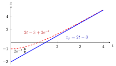
The figure uses the polynomial-forcing example below. Besides $x_p=2t-3$$3$, the function $2t-3+2\mathrm{e}^{-t}$ also satisfies $x''+3x'+2x=4t$$4t$, since $2\mathrm{e}^{-t}$ solves the homogeneous equation ($r=$$r=-1$ is a root of $r^2+3r+2$$2$). The gap between the two curves is exactly this homogeneous solution; here it dies out, so both curves follow the same forced response for large $t$.

This mirrors linear algebra: for a homogeneous and inhomogeneous system $A\boldsymbol{x}=\boldsymbol{b}$$\mathbf{b}$, one solution of the inhomogeneous system plus the null space gives all solutions. Here $L$ is linear, so the same structure holds; see general solution of a linear ODE.

For first-order equations a particular solution can always be computed with an integrating factor. For constant coefficients and forcing of polynomial, exponential, sine or cosine type, the method of undetermined coefficients is quicker: guess a function of the same type as $g$ with unknown coefficients and match terms. If the guess already solves the homogeneous equation (resonance), it must be multiplied by $t$; forgetting this leads to the impossible equation $0=g$$g$.

Key Results¶

• If $x_{p,1}$ and $x_{p,2}$ are particular solutions, then $x_{p,1}-x_{p,2}$ solves $L[x]=0$$0$.
• Superposition: if $L[x_1]=g_1$ and $L[x_2]=g_2$$g_2$, then $L[x_1+x_2]=g_1+g_2$$g_2$.
• Constant coefficients and constant forcing $g\equiv c$ with $a_0\neq0$$0$: $x_p=c/a_0$$c/a_0$, the equilibrium of the equation.
• Exponential forcing $g=k\mathrm{e}^{st}$ with constant coefficients: if $p(s)\neq0$ for the characteristic polynomial $p$, then $x_p=\frac{k}{p(s)}\mathrm{e}^{st}$$\frac{k}{p(s)}{\mathrm{e}}^{st}$; if $s$ is a simple root of $p$, then $x_p=\frac{k}{p'(s)}t\mathrm{e}^{st}$$\frac{k}{p^{\prime }(s)}t{\mathrm{e}}^{st}$.
• In general, if the exponent $s$ (or $\alpha\pm\mathrm{i}\beta$ for $\mathrm{e}^{\alpha t}\cos\beta t$, $\mathrm{e}^{\alpha t}\sin\beta t$) is a root of multiplicity $m$, the trial function is multiplied by $t^m$.
• Vector case: for $\boldsymbol{x}'=A\boldsymbol{x}+\boldsymbol{b}$ with constant $\boldsymbol{b}$ and invertible $A$, the constant $\boldsymbol{x}_p=-A^{-1}\boldsymbol{b}$ is a particular solution.

Examples¶

Polynomial forcing. For the second-order differential equation $x''+3x'+2x=4t$$4t$, try $x_p=At+B$$B$: then $3A+2At+2B=4t$$4t$, so $A=2$ and $B=-3$$-3$. Check: $0+3\cdot2+2(2t-3)=4t$$4t$.

Exponential forcing. $x''-x'-6x=\mathrm{e}^{t}$ with $p(r)=r^2-r-6$$6$: $p(1)=-6\neq0$$0$, so $x_p=-\tfrac{1}{6}\mathrm{e}^{t}$$-\frac{1}{6}{\mathrm{e}}^t$.

Resonance. $x''-x'-6x=\mathrm{e}^{3t}$${\mathrm{e}}^{3t}$: $3$ is a simple root of $p$, so try $x_p=At\mathrm{e}^{3t}$$At{\mathrm{e}}^{3t}$. Then $x_p'=A(1+3t)\mathrm{e}^{3t}$$3t){\mathrm{e}}^{3t}$, $x_p''=A(6+9t)\mathrm{e}^{3t}$ and $L[x_p]=A\big[(6+9t)-(1+3t)-6t\big]\mathrm{e}^{3t}=5A\mathrm{e}^{3t}$$5A{\mathrm{e}}^{3t}$, so $A=\tfrac{1}{5}$$\frac{1}{5}$, in line with $p'(3)=5$$5$.

Sinusoidal forcing. $x''+x=\cos2t$$\cos 2t$: try $A\cos2t$; $-4A+A=1$ gives $x_p=-\tfrac{1}{3}\cos2t$$-\frac{1}{3}\cos 2t$. For $x''+x=\cos t$ the frequency matches the roots $\pm\mathrm{i}$, and $x_p=\tfrac{t}{2}\sin t$ (check: $x_p''=\cos t-\tfrac{t}{2}\sin t$$\frac{t}{2}\sin t$).

Prerequisites¶

• Second-Order Differential Equation
• Characteristic Equation for a Differential Equation
• Integrating Factor
• Homogeneous and Inhomogeneous Systems

Related Concepts¶

• General Solution of a Linear ODE
• Equilibrium of a Differential Equation
• Linear Vector ODE
• Stability of Solutions of Higher-Order ODEs

Sources¶

• Math V: Advanced Linear Algebra · Week 4

Aliases: particular solution, particular integral Keywords: x_p, method of undetermined coefficients, trial solution, resonance, forcing term Symbols: alpha, beta

Last updated: 22 October 2026 19:04