Second-Order Linear Difference Equation¶

Definition¶

A second-order linear difference equation with constant coefficients is

for $t=0,1,2,\ldots$$0,1,2,\dots$, with real constants $a_1$ and $a_0\ne0$ and a given sequence $(g_t)$. Its homogeneous version has $g_t=0$$0$. Write $r_1,r_2$ for the roots of the characteristic polynomial $p(r)=r^2+a_1r+a_0$$a_0$. The general solution of the homogeneous equation is, with arbitrary constants $c_1,c_2$:

• distinct real roots $r_1\ne r_2$$r_2$: $x_t=c_1r_1^t+c_2r_2^t$$c_2{r}_2^t$;
• a repeated root $r_1=r_2=r$$r$: $x_t=(c_1+c_2t)\,r^t$$c_{2}t)r^t$;
• nonreal roots $\rho \mathrm{e}^{\pm\mathrm{i}\theta}$ with $\rho>0$$0$, $0<\theta<\pi$$\pi$: $x_t=\rho^t\big(c_1\cos(\theta t)+c_2\sin(\theta t)\big)$$c_2\sin (\theta t))$.

Interpretation¶

The next value depends on the two most recent values, so two initial values $x_0,x_1$ are needed to fix a solution; they determine $c_1,c_2$. Unlike the first-order case, where the only oscillation is the sign alternation caused by $a<0$$0$, the solutions can oscillate with any frequency, because the roots may be nonreal complex numbers. The real form in the third case comes from combining the conjugate solutions $(\rho \mathrm{e}^{\mathrm{i}\theta})^t$ and $(\rho \mathrm{e}^{-\mathrm{i}\theta})^t$; $\rho$ sets growth or decay and $\theta$ the frequency.

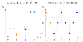
In both panels the two orange values $x_0,x_1$ are given, and every later value follows from the recursion. On the left, the distinct roots $2$ and $3$ of the first example below give $x_t=2\cdot3^t-2^t$$2^t$, which grows like $3^t$. On the right, the nonreal roots $\pm\mathrm{i}$ ($\rho =$$\rho=1$$1$, $\theta=\pi/2$$\pi /2$) with $x_0=1$$1$, $x_1=0$ give $c_1=1$$1$, $c_2=0$$0$, so $x_t=\cos(\pi t/2)$$\cos (\pi t/2)$: an oscillation with frequency set by $\theta$ and constant amplitude $\rho^t=1$$1$.

The repeated-root case is a standard trap: $c_1r^t+c_2r^t$ is only a one-parameter family, so a second solution $t\,r^t$ is needed.

For a constant input $g_t=b$ with $p(1)=1+a_1+a_0\ne0$$0$, the constant $x^*=b/p(1)$ is a particular solution, and the general solution is $x^*$ plus the homogeneous solution.

Key Results¶

• Every choice of $x_0,x_1$ gives exactly one solution; the homogeneous solutions form a two-dimensional space with the basis of solutions listed above.
• General solution of the inhomogeneous equation = one particular solution + general homogeneous solution.
• Root relations: $r_1+r_2=-a_1$ and $r_1r_2=a_0$$a_0$; the roots are nonreal if and only if $a_1^2<4a_0$$4a_0$.
• If $1$ is a simple root of $p$ (so $p(1)=0$$0$, $2+a_1\ne0$$0$) and $g_t=b\ne0$$0$, there is no equilibrium; $x_t=Ct$ with $C=b/(2+a_1)$ is a particular solution. If instead $b=0$$0$, every constant sequence is an equilibrium.
• All solutions tend to $x^*$ if and only if $\lvert r_1\rvert<1$ and $\lvert r_2\rvert<1$$1$, equivalently $\lvert a_0\rvert<1$ and $\lvert a_1\rvert<1+a_0$ (see stability).

Examples¶

Distinct roots. $x_{t+2}-5x_{t+1}+6x_t=0$$0$, $x_0=1$$1$, $x_1=4$$4$. Then $p(r)=(r-2)(r-3)$$3)$, so $x_t=c_12^t+c_23^t$ with $c_1+c_2=1$$1$, $2c_1+3c_2=4$$4$, giving $c_2=2$$2$, $c_1=-1$$-1$: $x_t=2\cdot3^t-2^t$$2^t$. Check: $x_2=18-4=14=5\cdot4-6\cdot1$$1$.

Constant input. $x_{t+2}-5x_{t+1}+6x_t=4$$4$: $p(1)=2$$2$, so $x^*=2$ and $x_t=2+c_12^t+c_23^t$$c_2{3}^t$.

Complex roots. $x_{t+2}+x_t=0$ has $p(r)=r^2+1$ with roots $\pm\mathrm{i}=\mathrm{e}^{\pm\mathrm{i}\pi/2}$${\mathrm{e}}^{\pm \mathrm{i}\pi /2}$, so $\rho=1$$1$, $\theta=\pi/2$ and $x_t=c_1\cos(\pi t/2)+c_2\sin(\pi t/2)$$c_2\sin (\pi t/2)$. With $x_0=1$$1$, $x_1=0$$0$: $1,0,-1,0,1,\ldots$, period $4$, neither growing nor decaying.

Prerequisites¶

• Difference Equation
• First-Order Linear Difference Equation
• Complex Number

Related Concepts¶

• Characteristic Polynomial for a Difference Equation
• Basis of Solutions of a Difference Equation
• Higher-Order Linear Difference Equation
• Second-Order Differential Equation

Sources¶

• Math V: Advanced Linear Algebra · Week 2

Aliases: Second Order Linear Difference Equation, second-order linear recurrence, linear second-order difference equation, linear difference equation of order two Keywords: x_{t+2} + a_1 x_{t+1} + a_0 x_t = g_t, two initial values, distinct, repeated and complex roots, r^t and t r^t, rho^t cos(theta t) Symbols: pi, rho, theta

Last updated: 27 October 2026 11:52