Stability of Solutions of Higher-Order ODEs¶

Proposition¶

Consider the linear ordinary differential equation (ODE) with constant real coefficients

x^{(n)}(t)+a_{n-1}x^{(n-1)}(t)+\dots +a_1x'(t)+a_0x(t)=g(t),

with $x'(t)=\dfrac{\mathrm{d}x}{\mathrm{d}t}(t)$ and characteristic equation $p(r)=r^n+a_{n-1}r^{n-1}+\dots+a_0=0$ $0$ . For the homogeneous equation ( $g \equiv$ $g\equiv0$ $0$ ):

Every solution satisfies $x(t)\to0$ as $t\to\infty$ if and only if every root of $p$ has negative real part. The equation is then called asymptotically stable.
If some root has positive real part, some solutions are unbounded: the equation is unstable.
If all roots have real part $\leq0$ $0$ , all solutions are bounded on $[0,\infty)$ if and only if every root with real part $0$ is simple; the equation is then called stable. A repeated root on the imaginary axis gives unbounded terms such as $t$ or $t\cos\beta t$ .

For constant $g\equiv c$ with $a_0\neq0$ $0$ , every solution tends to the equilibrium $c/a_0$ if and only if all roots have negative real part.

In Math V, stable means that all solutions stay bounded, and asymptotically stable that they all converge (case 1). A simple root on the imaginary axis therefore gives a stable equation that is not asymptotically stable.

Interpretation¶

By the general solution of a linear ODE, every homogeneous solution is a combination of terms $t^j\mathrm{e}^{rt}$ , one family for each root $r=\alpha+\mathrm{i}\beta$ $i β$ . With Euler's formula, $|t^j\mathrm{e}^{rt}|=t^j\mathrm{e}^{\alpha t}$ $t^{j} e^{α t}$ : the oscillation $\mathrm{e}^{\mathrm{i}\beta t}$ has modulus $1$ , and only $\alpha$ decides growth or decay. Exponential decay beats any polynomial factor $t^j$ , so $\alpha<0$ is enough.

In the complex plane the open left half-plane is shaded; the roots −1 and −2 lie inside it, ±2i lie on the imaginary axis, and 1 ± 2i and a double root 0 are unstable.

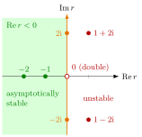
The figure places the characteristic roots of the examples below in the complex plane. The roots $-1,-2$ of $x''+3x'+2x=4$ lie in the shaded half-plane $\operatorname{Re} r<0$ $0$ , so every solution converges. The simple roots $\pm2\mathrm{i}$ of $x''+4x=0$ lie on the imaginary axis: solutions stay bounded but do not decay. The roots $1\pm2\mathrm{i}$ of $x''-2x'+5x=0$ lie to the right, and the double root $0$ of $x''=0$ lies on the axis but is repeated; both give unbounded solutions.

The criterion is the continuous-time counterpart of stability of an equilibrium: writing the equation as a first-order system, the roots are the eigenvalues of the companion matrix, and "negative real part" plays the role of $f'(x^*)<0$ $0$ . For difference equations the boundary is the unit circle $|\lambda|=1$ $1$ , not the imaginary axis; see stability of a scalar difference equation.

Typical mistakes: requiring only real roots to be negative and ignoring complex ones; treating purely imaginary roots as stable in the asymptotic sense; and concluding stability from positive coefficients alone when $n\geq3$ $3$ .

Key Results¶

Order 2: $x''+a_1x'+a_0x=0$ is asymptotically stable if and only if $a_1>0$ and $a_0>0$ (the roots have sum $-a_1$ and product $a_0$ ).
For any $n$ , positive coefficients $a_0,\dots,a_{n-1}$ are necessary for asymptotic stability, but not sufficient when $n\geq3$ $3$ .
Stability is a property of the homogeneous part and does not depend on $g$ : all solutions $x=x_p+x_h$ satisfy $x(t)-x_p(t)\to0$ if and only if all roots have negative real part.
The same test applies to the first-order system form: its companion matrix has the roots of $p$ as eigenvalues, as for the linear vector ODE.

Beyond the course

Many textbooks state the Routh-Hurwitz criterion, which decides from the coefficients alone whether all roots have negative real part. It is not part of Math V.

Examples¶

Asymptotically stable with forcing. $x''+3x'+2x=4$ $4$ : roots $-1,-2$ , and the particular solution is $x_p=2$ $2$ . Every solution $2+c_1\mathrm{e}^{-t}+c_2\mathrm{e}^{-2t}$ tends to $2$ .

Pure oscillation. $x''+4x=0$ $0$ : roots $\pm2\mathrm{i}$ , solutions $c_1\cos2t+c_2\sin2t$ are bounded but do not tend to $0$ : stable, not asymptotically stable.

Growing oscillation. $x''-2x'+5x=0$ $0$ : $r=1\pm2\mathrm{i}$ $2 i$ , solutions $\mathrm{e}^{t}(c_1\cos2t+c_2\sin2t)$ $c_{2} sin 2 t)$ : unstable, matching $a_1=-2<0$ $0$ .

Double root at zero. $x''=0$ $0$ : $r=0$ twice, solutions $c_1+c_2t$ $c_{2} t$ , unbounded: unstable although no root has positive real part.

Positive coefficients are not enough. $r^3+r^2+r+1=(r+1)(r^2+1)$ has roots $-1,\pm\mathrm{i}$ . All coefficients are positive, yet the simple roots $\pm\mathrm{i}$ lie on the imaginary axis: stable, not asymptotically stable.

Prerequisites¶

Sources¶

Math V: Advanced Linear Algebra · Week 4

Aliases: Stability of Solutions of Higher Order ODEs, stability of a linear ODE, asymptotic stability of a higher-order ODE Keywords: negative real part, characteristic roots, Routh-Hurwitz, a_1>0, a_0>0, resonance on the imaginary axis Symbols: alpha, beta, infinity, lambda

Last updated: 27 October 2026 11:52