Skip to content

System of Differential Equations


Definition

A system of differential equations consists of nn first-order differential equations for nn unknown functions x1(t),…,xn(t)x_1(t),\dots,x_n(t). For i=1,…,ni=1,\dots,n,

xi′(t)=fi(t,x1(t),…,xn(t)),x_i'(t)=f_i\big(t,x_1(t),\dots,x_n(t)\big),

where xi′(t)=dxidt(t)x_i'(t)=\dfrac{\mathrm{d}x_i}{\mathrm{d}t}(t). With the state vector x(t)=(x1(t),…,xn(t))⊤\boldsymbol{x}(t)=\big(x_1(t),\dots,x_n(t)\big)^{\top} it reads x′(t)=f(t,x(t))\boldsymbol{x}'(t)=\boldsymbol{f}\big(t,\boldsymbol{x}(t)\big). The system is linear if

x′(t)=A(t) x(t)+b(t)\boldsymbol{x}'(t)=A(t)\,\boldsymbol{x}(t)+\boldsymbol{b}(t)

for an n×nn\times n matrix function A(t)A(t) and a vector function b(t)\boldsymbol{b}(t); it is coupled if some xi′x_i' depends on some xjx_j with j≠ij\neq i. An initial value problem prescribes the whole vector x(t0)∈Rn\boldsymbol{x}(t_0)\in\mathbb{R}^n.


Interpretation

A system describes several interacting quantities, such as two competing populations or prices in linked markets. In the linear case the matrix product AxA\boldsymbol{x} packs all couplings into one coefficient matrix; the entry aija_{ij} measures how xjx_j affects the rate of change of xix_i.

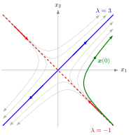
In the phase plane of the coupled example, solutions move out along the line through (1,1) and in along the line through (1,−1), and the green curve passes through x(0) = (3,1).

The figure shows the coupled example below in the (x1,x2)(x_1,x_2) plane. Along the eigenvector (1,1)⊤(1,1)^{\top} (blue, λ=3\lambda=3) solutions move outwards like e3t\mathrm{e}^{3t}, along (1,−1)⊤(1,-1)^{\top} (red, λ=−1\lambda=-1) they move inwards like e−t\mathrm{e}^{-t}, and every other solution (grey) combines the two. The green curve is the solution with x(0)=(3,1)⊤\boldsymbol{x}(0)=(3,1)^{\top}: it comes in near the (1,−1)⊤(1,-1)^{\top} line and then leaves in the (1,1)⊤(1,1)^{\top} direction. Neither coordinate can be solved on its own, but in eigenvector coordinates the two motions separate.

Every scalar equation of order nn is a first-order system in disguise: with y1=xy_1=x, y2=x′y_2=x', ..., yn=x(n−1)y_n=x^{(n-1)} the equation x(n)=f(t,x,…,x(n−1))x^{(n)}=f(t,x,\dots,x^{(n-1)}) becomes y1′=y2, …, yn−1′=yn, yn′=f(t,y1,…,yn)y_1'=y_2,\ \dots,\ y_{n-1}'=y_n,\ y_n'=f(t,y_1,\dots,y_n). For a second-order differential equation this gives a two-dimensional system. So first-order systems are the general framework, and one theory covers all orders.

Coupling is what makes systems harder than nn separate scalar equations. For constant, diagonalizable AA the eigenvalues and eigenvectors remove it: a coordinate change along eigenvectors turns the system into decoupled scalar equations. A common error is to solve each row as if the other variables were constants. The discrete-time counterpart is the system of linear difference equations xt+1=Axt\boldsymbol{x}_{t+1}=A\boldsymbol{x}_t.


Key Results

  • For a linear system with continuous A(t),b(t)A(t),\boldsymbol{b}(t) on an interval II, each initial value problem has exactly one solution on II.
  • If b=0\boldsymbol{b}=\boldsymbol{0} and AA is constant and diagonalizable, A=PDP−1A=PDP^{-1} (diagonalization), then y=P−1x\boldsymbol{y}=P^{-1}\boldsymbol{x} satisfies y′=Dy\boldsymbol{y}'=D\boldsymbol{y}, i.e. yi′=λiyiy_i'=\lambda_iy_i, so yi(t)=yi(0)eλity_i(t)=y_i(0)\mathrm{e}^{\lambda_it}.
  • In that case x(t)=∑icieλitvi\displaystyle \boldsymbol{x}(t)=\sum_i c_i\mathrm{e}^{\lambda_it}\boldsymbol{v}_i, with vi\boldsymbol{v}_i the columns of PP; for any constant AA, x(t)=eAtx(0)\boldsymbol{x}(t)=\mathrm{e}^{At}\boldsymbol{x}(0) with the matrix exponential.
  • The companion matrix of x′′+a1x′+a0x=0x''+a_1x'+a_0x=0 is (01−a0−a1)\begin{pmatrix}0&1\\-a_0&-a_1\end{pmatrix}, with characteristic polynomial λ2+a1λ+a0\lambda^2+a_1\lambda+a_0.

Examples

Coupled linear system. x1′=x1+2x2x_1'=x_1+2x_2, x2′=2x1+x2x_2'=2x_1+x_2, so A=(1221)A=\begin{pmatrix}1&2\\2&1\end{pmatrix}. Eigenpairs: A(1,1)⊤=3(1,1)⊤A(1,1)^{\top}=3(1,1)^{\top} and A(1,−1)⊤=−(1,−1)⊤A(1,-1)^{\top}=-(1,-1)^{\top}. Hence

x(t)=c1e3t(11)+c2e−t(1−1).\boldsymbol{x}(t)=c_1\mathrm{e}^{3t}\begin{pmatrix}1\\1\end{pmatrix}+c_2\mathrm{e}^{-t}\begin{pmatrix}1\\-1\end{pmatrix}.

With x(0)=(3,1)⊤\boldsymbol{x}(0)=(3,1)^{\top}: c1+c2=3c_1+c_2=3, c1−c2=1c_1-c_2=1, so c1=2c_1=2, c2=1c_2=1 and x(t)=(2e3t+e−t, 2e3t−e−t)⊤\boldsymbol{x}(t)=\big(2\mathrm{e}^{3t}+\mathrm{e}^{-t},\ 2\mathrm{e}^{3t}-\mathrm{e}^{-t}\big)^{\top}.

Reduction of order. x′′+3x′+2x=0x''+3x'+2x=0 becomes, with y1=xy_1=x, y2=x′y_2=x', the system y′=(01−2−3)y\boldsymbol{y}'=\begin{pmatrix}0&1\\-2&-3\end{pmatrix}\boldsymbol{y}, whose eigenvalues −1,−2-1,-2 are the roots of r2+3r+2r^2+3r+2.

Decoupled system. x1′=−x1x_1'=-x_1, x2′=4x2x_2'=4x_2 has diagonal AA and solution (x1(0)e−t, x2(0)e4t)⊤\big(x_1(0)\mathrm{e}^{-t},\ x_2(0)\mathrm{e}^{4t}\big)^{\top}.


Prerequisites


Sources

Aliases: system of ODEs, coupled differential equations, system of ordinary differential equations, ODE system, vector differential equation Keywords: x'(t)=f(t,x(t)), first-order system, companion matrix, decoupling, state vector Symbols: element of, lambda, real numbers, sum

Last updated: 17 October 2026 21:53