General Solution of a Linear ODE¶

Proposition¶

Let $a_0,\dots,a_{n-1}$ and $g$ be continuous on an interval $I$ , write $x'(t)=\dfrac{\mathrm{d}x}{\mathrm{d}t}(t)$ $\frac{d x}{d t} (t)$ , and let

L[x]=x^{(n)}+a_{n-1}(t)x^{(n-1)}+\dots +a_1(t)x'+a_0(t)x.

The solutions of the homogeneous equation $L[x]=0$ on $I$ form a vector space $S_0$ of dimension $n$ .
If $x_p$ is a particular solution of $L[x]=g$ $g$ , then the set of all solutions of $L[x]=g$ is $\{x_p\}+S_0$ $S_{0}$ .

Hence, for any basis $x_1,\dots,x_n$ of $S_0$ , the general solution of the linear ordinary differential equation (ODE) $L[x]=g$ is

x(t)=x_p(t)+c_1x_1(t)+\dots+c_nx_n(t),

where $c_1,\dots,c_n\in\mathbb{R}$ $R$ , and $n$ initial conditions $x(t_0),x'(t_0),\dots,x^{(n-1)}(t_0)$ determine $c_1,\dots,c_n$ uniquely.

Interpretation¶

The map $L$ is linear, so $S_0$ is its kernel and the solution set of $L[x]=g$ is a shifted copy of that kernel. This is the same structure as for homogeneous and inhomogeneous systems $A\boldsymbol{x}=\boldsymbol{b}$ in Math II, and the solution set is an affine subspace, not a subspace, when $g\not\equiv0$ $0$ .

The solution x(t) of the example starting at 0 with zero slope, the dashed particular solution 2t - 3, and the homogeneous part 4e^(-t) - e^(-2t) decaying from 3 towards 0.

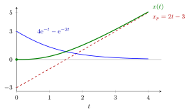
The figure plots the second-order example $x''+3x'+2x=4t$ with $x(0)=x'(0)=0$ $0$ . The green solution $x(t)=4\mathrm{e}^{-t}-\mathrm{e}^{-2t}+2t-3$ is the dashed particular solution $x_p=2t-3$ plus the blue element $4\mathrm{e}^{-t}-\mathrm{e}^{-2t}$ of $S_0$ . The constants $c_1=4$ $4$ , $c_2=-1$ are fitted to the full sum, which is why $x$ starts at $0$ with zero slope while $x_p$ starts at $-3$ . As the homogeneous part decays, $x(t)$ approaches $x_p(t)$ .

The proof of part 2 is one line: if $L[x]=g$ then $L[x-x_p]=g-g=0$ $0$ , so $x-x_p\in S_0$ $S_{0}$ . The dimension count in part 1 uses uniqueness of solutions: the map sending a solution to its initial data $\big(x(t_0),\dots,x^{(n-1)}(t_0)\big)\in\mathbb{R}^n$ is a linear bijection.

Common errors: fitting the initial conditions to the homogeneous part before adding $x_p$ (the constants must be fitted to the full sum); and assuming the sum of two particular solutions is again a particular solution (it solves $L[x]=2g$ $2 g$ ).

Key Results¶

$n$ solutions $x_1,\dots,x_n$ of $L[x]=0$ form a basis of $S_0$ if and only if their initial-data vectors $\big(x_i(t_0),x_i'(t_0),\dots,x_i^{(n-1)}(t_0)\big)$ are linearly independent for one (equivalently every) $t_0\in I$ $I$ .
For constant coefficients, the roots of the characteristic equation supply such a basis.
The same structure holds for systems: all solutions of $\boldsymbol{x}'=A\boldsymbol{x}+\boldsymbol{b}(t)$ are $\boldsymbol{x}_p$ plus the $n$ -dimensional solution space of $\boldsymbol{x}'=A\boldsymbol{x}$ $A x$ ; see linear vector ODE.
For constant $A$ , the general solution is $\boldsymbol{x}(t)=\mathrm{e}^{A(t-t_0)}\boldsymbol{x}(t_0)+\int_{t_0}^{t}\mathrm{e}^{A(t-s)}\boldsymbol{b}(s)\,\mathrm{d}s$ $\int_{t_{0}}^{t} e^{A (t - s)} b (s) d s$ , using the matrix exponential.

Beyond the course

Many differential-equations textbooks test this independence with the Wronskian, the determinant of the matrix whose columns are the initial-data vectors at $t$ . Math V does not use it: checking the initial-data vectors at one $t_0$ is enough.

Examples¶

Second-order initial value problem. $x''+3x'+2x=4t$ $4 t$ , $x(0)=0$ $0$ , $x'(0)=0$ $0$ . Homogeneous basis from $r^2+3r+2=(r+1)(r+2)$ $2)$ : $\mathrm{e}^{-t}$ , $\mathrm{e}^{-2t}$ . A particular solution is $2t-3$ $3$ . So $x=c_1\mathrm{e}^{-t}+c_2\mathrm{e}^{-2t}+2t-3$ $3$ . The conditions give $c_1+c_2=3$ and $-c_1-2c_2+2=0$ $0$ , hence $c_2=-1$ $- 1$ , $c_1=4$ $4$ :

x(t)=4\mathrm{e}^{-t}-\mathrm{e}^{-2t}+2t-3.

Check: $x(0)=4-1-3=0$ and $x'(0)=-4+2+2=0$ $0$ .

Independence check. At $t_0=0$ the initial-data vectors of $\mathrm{e}^{-t}$ and $\mathrm{e}^{-2t}$ are $(1,-1)$ and $(1,-2)$ , which are linearly independent, so $\mathrm{e}^{-t},\mathrm{e}^{-2t}$ form a basis of $S_0$ .

First order. $x'=-2x+6$ $6$ : $S_0=\{C\mathrm{e}^{-2t}\}$ has dimension 1 and $x_p=3$ $3$ , so $x(t)=3+C\mathrm{e}^{-2t}$ $C e^{- 2 t}$ .

Prerequisites¶

Sources¶

Math V: Advanced Linear Algebra · Week 4

Aliases: general solution Keywords: superposition principle, x = x_p + x_h, fundamental set of solutions, solution space, Wronskian, homogeneous solution Symbols: element of, integral, real numbers

Last updated: 22 October 2026 19:04